Network anomaly detection using deep learning techniques

Mohammad Kazim Hooshmand |Doreswamy Hosahalli

Department of Computer Science,Mangalore University,Mangalore,India

Abstract Convolutional neural networks (CNNs) are the specific architecture of feed-forward artificial neural networks.It is the de-facto standard for various operations in machine learning and computer vision.To transform this performance towards the task of network anomaly detection in cyber-security,this study proposes a model using one-dimensional CNN architecture.The authors' approach divides network traffic data into transmission control protocol (TCP),user datagram protocol (UDP),and OTHER protocol categories in the first phase,then each category is treated independently.Before training the model,feature selection is performed using the Chisquare technique,and then,over-sampling is conducted using the synthetic minority over-sampling technique to tackle a class imbalance problem.The authors' method yields the weighted average f-score 0.85,0.97,0.86,and 0.78 for TCP,UDP,OTHER,and ALL categories,respectively.The model is tested on the UNSW-NB15 dataset.

KEYWORDS artificial intelligence,convolution,neural network,security

1|INTRODUCTION

Cyber-attacks are continuously evolving with the sophistication and advancement of hardware,software,and network topologies.Intrusion detection systems are highly recommended in defending the network from malicious cyber-attacks[1].Recent studies show that deep learning (DL) techniques are used in various areas such as natural language processing(NLP),speech recognition,computer vision,cyber-security etc.,because they have the capabilities of handling high-dimensional data with imbalanced classes and non-linear properties[2-4].A dataset is called imbalanced if a sample of one class contains more instances than the others[5].An imbalanced dataset can be binaryclass or multi-class.However,many conventional machine learning (ML) algorithms such as support vector machine(SVM),Naive Bayes (NB),decision tree (DT),random forest(RF),and many more are proposed by the previous studies for network anomaly detection[4,6-10],but the main limitation is that to evaluate the model performance,only well-balanced network traffic data is adopted.Most of the standard algorithms lead to a biased result towards the majority class in an imbalanced dataset because they tend to favour the majority class over the minority class.In such a condition,they will yield higher results for the majority classes and lower results for the minority ones [11,12].To overcome this limitation and to tackle nonlinear properties of datasets,the development of DL models with a combination of sampling techniques are encouraged.To resolve an imbalance issue,there are many sampling techniques.One of the most commonly used of such techniques is the synthetic minority over-sampling technique(SMOTE),which is proposed by Chawla [13].The SMOTE method generates additional synthetic samples from the minority class to balance the data.In this study,1-D convolutional neural network(CNN)architecture is trained on a sample of the newly generated UNSW-NB15 dataset.From feature visualisation of the UNSWNB15 dataset in Figure 1,we observe that the data distribution is different from protocol to protocol,overlap of classes and distribution are completelydifferent.This difference will impact the classifier's behaviour so that we split the data into different protocol categories first and then treated each one separately.On the other hand from Table 1,we can see that the data is very imbalanced,for example,‘worms’,‘shellcode’,‘backdoor’,and‘analysis’ are very less in terms of the number of instances compared to the other classes in all protocol categories.In addition to that,some classes do not exist under some protocols,for example,‘analysis’does not exist under user datagram protocol(UDP),and‘worms’and‘shellcode’do not exist under the‘OTHER’category.To tackle the issues of imbalance,we applied the SMOTE over-sampling technique on minority classes for each protocol category separately.The main steps that we followed in this study are data pre-processing,data division into protocols,feature selection using the Chi-square technique,over-sampling of minority classes using SMOTE technique,and applying 1-D CNN for multi-classification.

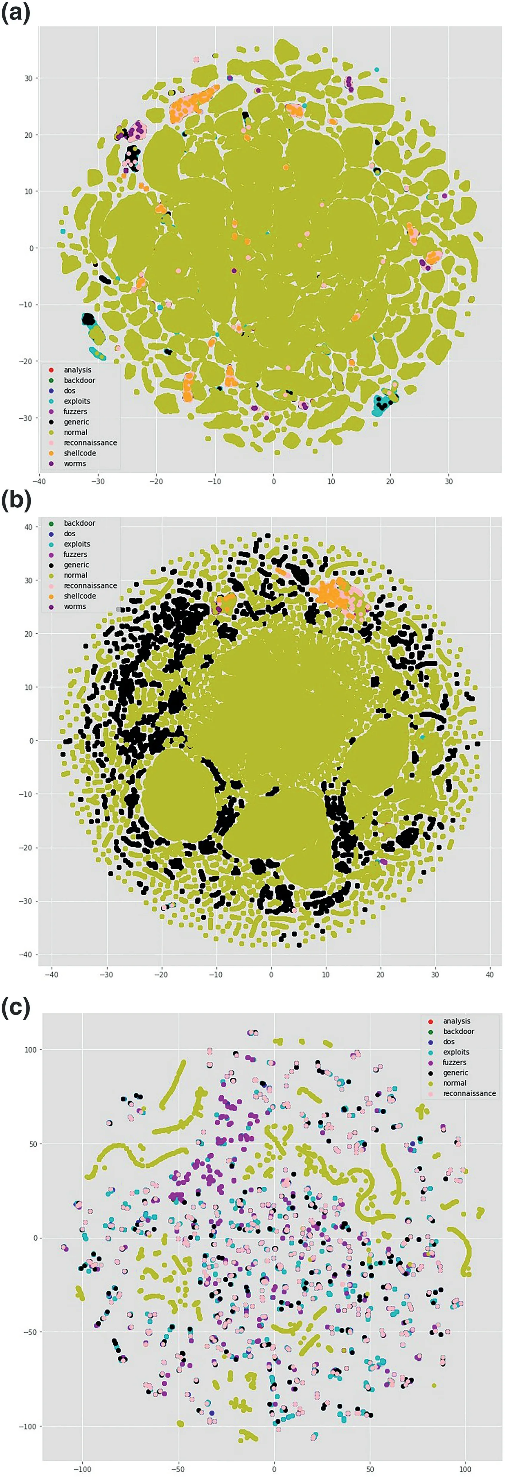
FIGURE 1 t-Distributed stochastic neighbour embedding (t-SNE)visualisation of full UNSW-NB15 dataset.(a) t-SNE visualisation of transmission control protocol;(b) t-SNE visualisation of user datagram protocol;(c) t-SNE visualisation of OTHER

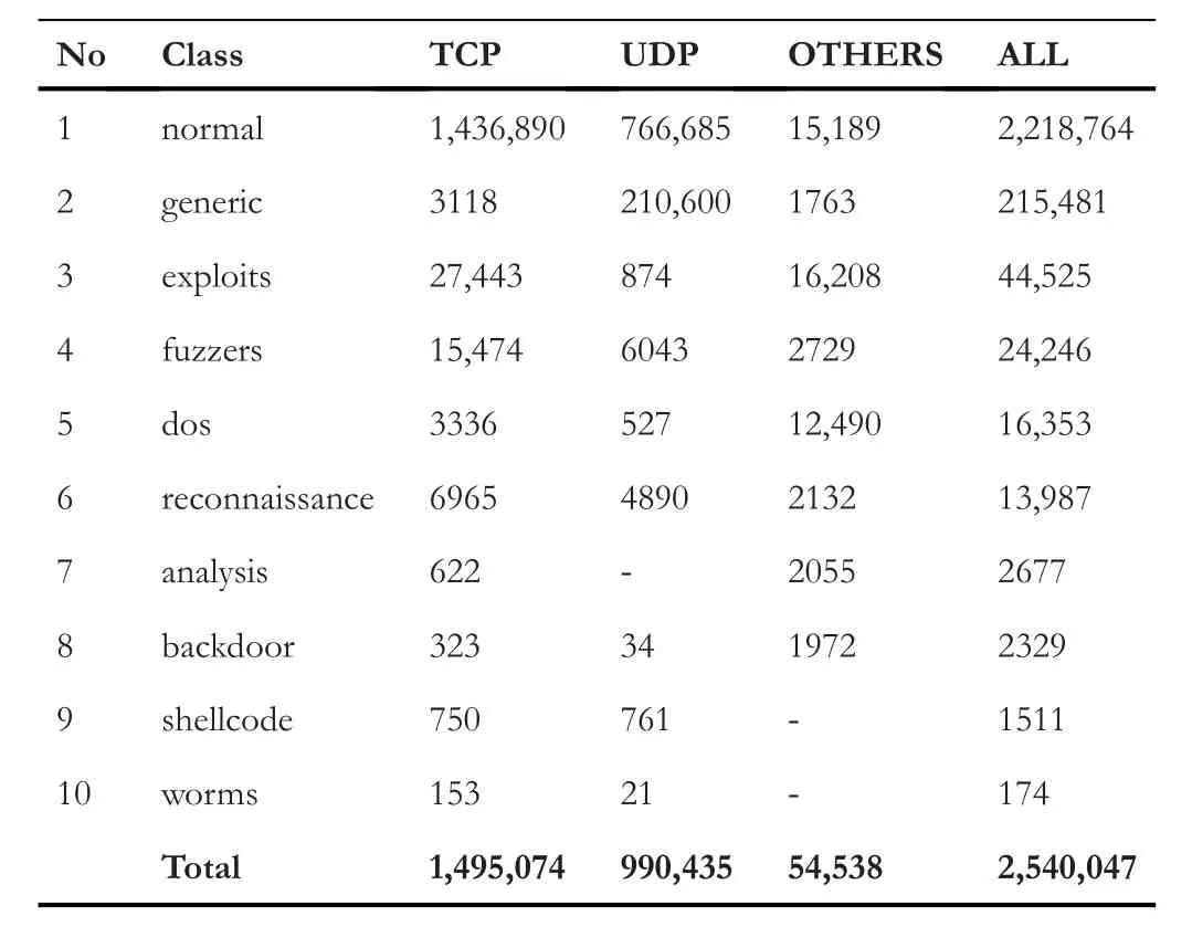
TABLE 1 Distribution of classes over different protocols in UNSWNB15

Overall,this study has made the following contributions in the field of cyber-security:

· By combining the SMOTE over-sampling technique and the 1-D CNN technique,the proposed model is able to classify minority classes of attacks with a higher accuracy rate.

· Features visualisation is conducted using at-distributed stochastic neighbour embedding (t-SNE) method prior to training the model.From Figure 1,we know that the distribution of different classes vary from protocol to protocol,so we divided the data into different protocol categories and then performed classification on each category as well as on the total data.We compared the results and observed that the model is performing better in protocol-wise multi-classification compared to all protocols combined.

The rest of this paper is arranged as follows:section 2 presents a summarised literature review;section 3 gives dataset descriptions;section 4 provides the proposed method;experimental results are discussed in section 5;result analysis and comparison are provided in section 6,and section 7 describes the conclusion and future work.

2|RELATED WORKS

In[3],the authors proposed three different CNN architectures(i.e.deep CNN,moderate CNN,and shallow CNN)for network anomaly detection.They conclude that the shallow CNN mostly yields better accuracy compared to the others.In [14],the authors proposed an intrusion detection model using CNN;the performance was evaluated on NSL-KDD(NSL-KDD Train+,NSL-KDD Test+) dataset in TensorFlow.They performed feature extraction and data pre-processing.Categorical features were encoded using a one-hot encoding technique;numeric variables were normalised using standard scalar,and then,the dataset was transformed into binary vectors with 464 variables.In the next step,those binary vectors were used to generate images with 8*8 grey-scale pixels,and finally,two CNN models GoogLeNet and ResNet-50 were used to identify the imageconversion category.The experimental results show that GoogLeNet and ResNet-50 scored 90.01% and 89.85% of the highestf-score,respectively.The parameters setting of this study is as follows:the number of epochs for both models was 100;the batch size was 62 for GoogLeNet and 256 for ResNet-50;the optimiser was gradient descent;the loss function was set to cross-entropy.

In the work done in [15],deep neural networks were proposed towards the task of anomaly detection.The result shows that DL methods are good for detecting anomalies in the software-defined network.

In [16],the authors employed simple CNN and hybrid CNN models.The simple model had multiple layers while the hybrid model was utilised using Long Short-Term Memory(LSTM) units,recurrent neural networks (RNNs),and gated recurrent units (GRUs) towards the task of network anomaly detection.The architecture includes an input layer,a hidden layer with one or more CNN layers followed by feed-forward networks (FFNs),and an output layer.The result of binary classification using the KDDCup99 dataset for both 1 layer and 2 layers showed a 99%f-score while the third layer CNN with LSTMs showed 98.7% accuracy for multi-classification.The model was evaluated using TensorFlow and the parameters used were as follows:inputs were set to 41*1;filters were 16,32,and 64;filter lengths were set to 3 and 5;the learning rate was given in the range of 0.01-0.5;the number of epochs was up to 1000.

In [17],the authors mentioned the usage of accelerated computing platform techniques with the aim of reducing training time and speeding up multi-classification of attacks.In[18],the authors proposed Stacked Auto-Encoders (SAE) for multi-classification of attacks and as well as for deep feature extraction.The result was good compared to existing approaches.In [19],the authors proposed RNN for multiclassification of attacks and the result was promising.They evaluated their approach on a sample of the NSL-KDD dataset.

3|UNSW‐NB15 DATASET

Earlier datasets such as DARPA 98/99,KDDCup99,and NSL-KDD were suffering from certain issues such as:(1)unavailability of knowledge on modern attacks'behaviours,(2)non-similarity of normal traffic existing in those datasets with a new pattern of normal traffic (because those datasets were generated decades ago),and(3)difference in the distribution of attack-types on training_set and testing_set[20].To overcome these issues of previous datasets,the UNSW-NB15 dataset was generated in 2015 [20-22] by Moustafa and Slay in the Australian Center for Cyber-Security lab(ACCS).The UNSWNB15 has 49 features including 2 labels (binary and multiclass).The attack categories and the classes are described in detail in [21,23] Table 1.

4|PROPOSED METHOD

The main steps of our proposed method are (1) data preprocessing,(2) dividing data into protocol categories such as transmission control protocol (TCP),UDP,OTHER,and ALL,(3) sampling (over-sampling the minority class and under-sampling the majority class),and (4) 1-D CNN-based classification.Figure 3 describes the architecture of our method.

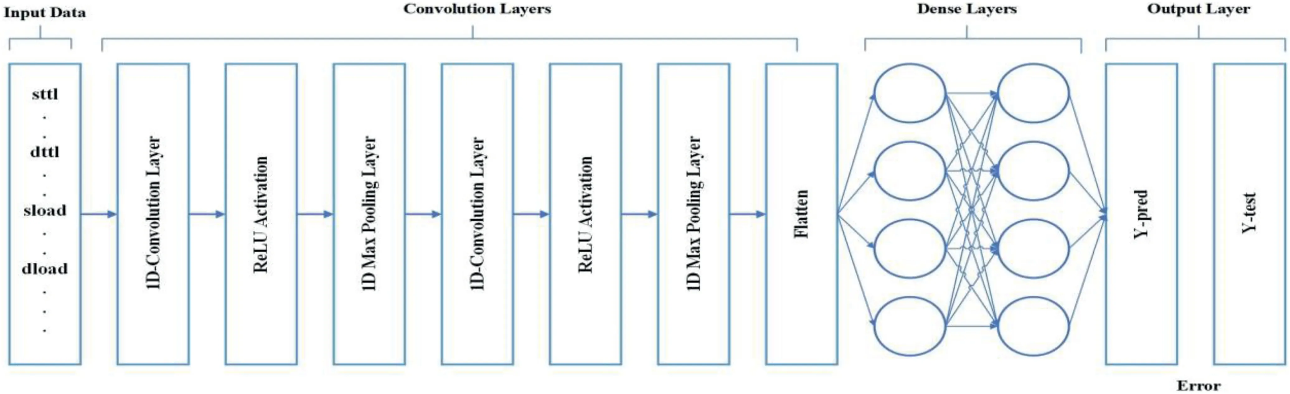
FIGURE 2 General architecture of 1-D Convolutional neural network

FIGURE 3 Architecture of the proposed model

4.1|Data pre‐processing

Switch information (‘srcip’,‘sport’,‘dstip’,‘dsport’) and time-related features (‘ltime’ and ‘stime’) are eliminated from the dataset because they are redundant features.Categorical features (‘proto’,‘state’,and ‘service’) have many values each.To encode these features,we apply a one-hot encoding technique,which will add a new variable for each value in each categorical feature.It will make the process very complex because it will add hundreds of new features to the data.To avoid that complexity,we categorise categorical values in such a way that feature values with more number of instances are kept as it is,and the remaining feature values with a lesser number of instances are put collectively under the ‘OTHER’ category.Reference to Table 2,we decided which feature value has to be kept as it is and which one has to be put under OTHER category.From the following categorization we can see that ‘state’ has FIN(finish),CON (connected),and INT (initiation).Similarly‘service’ has ‘-’ and domain name server (DNS).

· proto:‘TCP’,‘UDP’,‘OTHER’.

· state:‘FIN’,‘CON’,‘INT’,‘OTHER’.

· service:‘-’,‘DNS’,‘OTHER’.

TABLE 2 Categorical features

There are a few null values and spelling differences that exist in columns ‘ct_ftp_cmd’,‘is_ftp_login’,and‘ct_flw_http_mthd’,which are handled appropriately,and all null values under the ‘attack_cat’ feature are replaced with‘normal’.The nominal features are encoded and then thenormalisation is applied using the min_Max scaling technique.Equation(1)describes the way in which the min_Max method transforms values in the range of 0-1.

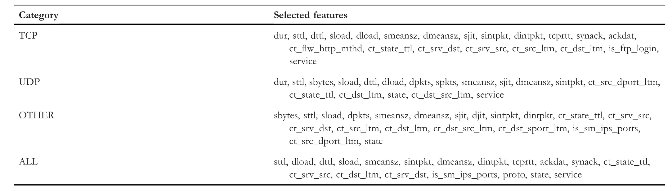
TABLE 3 Selected features of each category

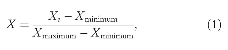
whereXstands for the normalised data,Xirepresents the original feature value,Xminimumis the minimum-value in feature,andXmaximumis the maximum-value in feature before the normalisation.

4.2|Data division

Prior to feature selection,we split the dataset based on different protocols.From Table 2,we know that TCP protocol contributes about 59%,UDP protocol covers about 39%,and the remaining protocols contribute about 2% of the dataset size.So,we split the data into three parts and treat each part as an independent data hereafter.The reason for dividing data into protocol-wise categories is that different protocol formats require a different set of features subsequently.

4.3|Feature selection

To eliminate less important features from a dataset,feature selection is necessary.We reduced number of features of all categories (TCP,UDP,OTHER,and ALL) to almost 50%using the Chi-square selection technique.The‘ALL’category is a combination of TCP,UDP,and OTHER after undersampling the majority class.Under-sampling and oversampling are explained in Section 4.4.

Detailed information on UNSW-NB15 and its categories of features is given in [23].Table 3 shows the list of selected features for each category.

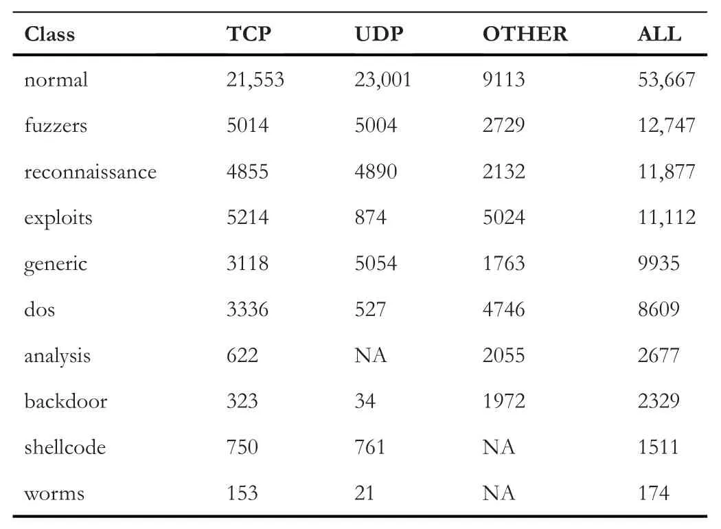
TABLE 4 Sample size of each protocol category

4.4|Sampling

Recently,different methods are proposed to solve the issue of class imbalance in a dataset.The methods are broadly grouped under two categories:algorithm level and data level[24].An algorithm-level approach works on modifying ML algorithms to accommodate the imbalanced dataset.Examples of such modifications can be cost-sensitive methods/cost error minimisation rather than accuracy rate maximisation [25].The data-level techniques are trying to rebalance the data class distribution either by decreasing the majority class or increasing the minority class.Various sampling methods exist,some of the examples can be random under-sampling,random over-sampling,direct over-sampling,SMOTE,and many others [24].Over-sampling techniques add some more instances to the minority class in the training set,the simplest method is random over-sampling [26] but the drawback is over-fitting [27].To overcome this problem,Chawla [13] proposed the SMOTE technique,which generates synthetic samples from the minority class.Samples created by the SMOTE technique are a linear combination of two identical samples from the minority class [13,26,28].The SMOTE over-sampling algorithm works as follows:LetSrepresent the size of a small class,considering a samplejof the small size class,andxjdenotes its feature vector such that,j∈{1,…,S}:

· Findkneighbours of the samplexjfrom allS(using the Euclidean Distance for example) and denoted it asxj(near),near∈{1,…,k}.

·xj(nn)sample is selected randomly from thekneighbours,and the random numberβ1between 0 and 1 is generated to synthesise a new samplexj1as in the equationxj1=xj+β1* (xj(nn)-xj).

· Step 2 is repeatedMtimes to synthesiseMnew samples:xj(new),new∈{1,…,M}.

In our case,we are under-sampling a few majority classes using random under-sampling.Then,we applied SMOTE over-sampling approach to over-sample the minority classes in the training set.Table 4 provides the size of each class sample with respect to protocol categories.

4.5|1‐D CNN

CNNs are the extension of feed-forward neural networks(FFNNs).The main components of CNNs are convolutional layer,non-linear activation function (e.g.Rectifier Linear Unit[ReLU]),and pooling layer (s) followed by one or more fully connected layers for the classification [29].Figure 2 illustrates the general architecture of 1-D CNN.

· Convolutional Layer:Its main task is to extract feature maps from vector input data using filters followed by activation functions such as ReLU,tanh etc.[16].The feature map calculation usingReLUand tanh non-linear functions are given in Equations (2) and (3),respectively.

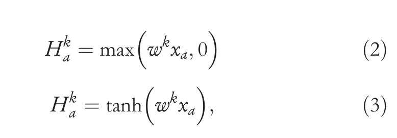
whereHkstands forkthfeature map,arepresents an index in the feature map,xastands for the input,andwkrepresents the weights.In this study,we used theReLUactivation function.

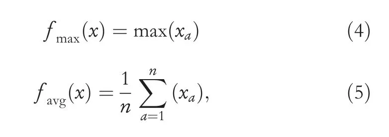
· Pooling Layer:Its main task is to under-sample each feature map's dimensions but keep the most informative feature map out of them.Hence,it reduces the computational cost and controls over-fitting in the model.The two commonly used pooling layers are average pooling and max pooling[30].In the max pooling,only the largest value from the window is selected by the function while the average pooling function considers the mean of all values in the window of the array currently covered by the kernel.The calculation methods of max pooling and average pooling are described in Equations (4) and (5),respectively.

wherexdescribes the vector of input data with an activation function,andndenotes a local pooling region.A detailed information on the pooling concept is given in[31,32].

· Fully Connected Layer:As the word itself describes,the fully connected means that every neuron of two consecutive layers are connected to each other.It is a multi-layer perceptron (MLP) that employs thesoftmaxfunction in the output layer.A fully connected layer is doing the same task that the standard artificial neural networks are doing,that is,to generate class scores from activations,which will be used for the classification [31].

· Activation Layer:It is the last layer of CNNs architecture that works similar to activation functions of the other neural networks.Some of the common activation functions employed in CNNs areReLU,sigmoid,andsoftmax.Our model uses asoftmaxactivation function for the classification problem of multi-class.Thesoftmaxfunction calculates the probabilities of each class and selects the highest value among the range of probability to produce the most accurate value for a class.The mathematical calculation ofsoftmaxis described in Equation (6).

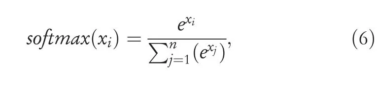
wherexdenotes an input.It applies the standard exponential function to each elementxiof the input vectorxand normalises these values by dividing by the sum of all these exponentials.Connecting all the above-mentioned points,the convolutional layer and pooling layer perform feature extraction duties while the fully connected layer is doing classification tasks.Figure 3 shows all the main steps of our proposed method,the CNN model contains three 1-D layers with aReLUactivation function followed by a flatten layer.The classification is done using two fully connected layers usingsoftmaxactivation.

5|EXPERIMENTAL RESULTS

The hardware and software configurations for our experiments are Windows 10 with an Intel®CoreTMi7-9700 central processing unit running at 3.00 GHz,8 processors,16 GB RAM,and 1 TB hard disk.Python 3.6 with libraries ofscikit learnandKeras[33,34] was utilised.As CNN is a parametrised function,so its performance fully depends on the optimal parameters,some of the parameters are the number of epochs,the number of hidden layers,the number of nodes in each layer etc.In [16],the authors claim that the lower learning rates have shown better results in differentiating the connection records using CNN.It is also mentioned that to attain the acceptable detection rate,the lower learning rate anticipate more number of epochs for lower frequency classes.In [35],the learning rate was assigned to 0.01 and theadamoptimiser was utilised for CNN architecture.In [1],the authors claim that,in the case of multi-classification,theReLUactivation function was performing better thansigmoidand tanh for 500 epochs.We have conducted different parameter adjustments in a tuning phase.The number of epochs was tested for 100-500,we decided on 500 because of its higher performance for all the categories of data (TCP,UDP,OTHER).Theoptimiseris set to ‘adam’ with default parameters,thelossis set to ‘categorical_crossentropy’,and themetricsare set toaccuracy,the batch size is 1,the number of nodes in each layer is 512,and the activation function isReLU.

The required time for running our model on the given configuration is calculated as follows:by calculating the required time for a single epoch execution and the number of epochs,we found that it takes approximately 7s to run one epoch.In the proposed method,we have considered 500 epochs,so the total time complexity of the model is 3500s.As per bigOnotations with respect to the number of loops and iterative approach,the complexity wasO(n).

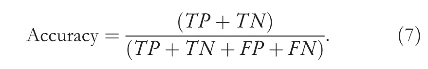
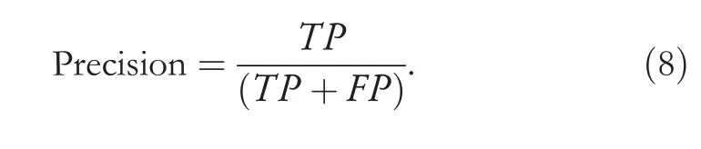
The metrics we used are Accuracy,Precision,Recall,andf-score.We used an accuracy measure to see the overall prediction of our model;it is good if you have a systematic dataset (false negatives false positives counts are close).Since our data has uneven class distribution,so accuracy will not give an accurate idea on every class,so we have used anf-score as well,which is best for uneven class data.Precision is used to be confident of our true positive value and Recall is used to get an understanding of the sensitivity of our prediction.All these metrics are explained and formulated in the Equations (7)-(10).

Accuracy:shows the ratio of truly detection over total transactions and calculated as

Precision:shows how many predicted intrusions by NIDs are actual intrusions and calculated as

Recall:it is the ratio of predicted intrusions versus all intrusions presented and calculated as

F-score:is a harmonic mean of Recall and Precision and gives a better measure of the accuracy and calculated as

where true positive is denoted by TP,false positive is shown by FP,TN is true negative,and FN is false negative.

Table 5 represents the confusion matrix of ‘TCP’ data,Table 6 shows the confusion matrix for ‘UDP’,and similarly,Tables 7 and 8 provide the confusion matrix for‘OTHER’and‘ALL’,respectively.From these confusion matrixes,we know that the accuracy for ‘ALL’ is lower for ‘backdoor’,‘dos’,‘exploits’,and ‘fuzzers’ compared to all the three categories(TCP,UDP,and OTHER).However,for ‘shellcode’ and‘analysis’,the accuracy is higher for ‘ALL’,and for the remaining classes,it is varying.Figure 4 provides a Precision score comparison for all categories.Figures 5 and 6 show a comparison of Recall andf-score,respectively.From Figure 4,we can see that the weighted average of precision for ‘ALL’ is 0.90,which is higher compared to precision of ‘TCP’ and‘OTHER’but lower than the precision of‘UDP’by 7%.From Figure 5,we can see that the weighted average of Recall for‘ALL’ is the lowest among all.As the weighted average of Recall score for‘ALL’is 0.76,which is lower by 20%from the leading score that is,‘UDP’,and lower by 10% and 8% from‘OTHER’ and ‘TCP’,respectively.Similarly from Figure 6,we observe that the‘ALL’category scores the lowest among all in terms off-score.Again the leading score belongs to‘UDP’with 0.97 followed by 0.86 and 0.85 for ‘OTHER’ and ‘TCP’ categories,respectively.Based on the comparison on Precision,Recall,andf-score,we can see that the score of ‘ALL’ is the lowest among all except for precision,which is higher than the score of ‘OTHER’ and ‘TCP’.It hints that treating protocolwise lead to better results.

6|RESULT ANALYSIS AND COMPARISON

6.1|Comparison

We have compared our method with two recent studies;Table 9 shows an overall performance comparison with the studies done in[1],for multi-classification in terms of accuracy,precision,recall,and f-score.We can see that our approach yields better results in terms of all the metrics.

Meanwhile,we compared our method with the study conducted in [36] for each class;the comparison is shown in Table 10.We observe that for the attack classes,our approach is performing much better except for the exploits and generic.However,in the case of normal,our method gets a lower result with a small percentage of 0.007.

TABLE 5 Confusion matrix for transmission control protocol

TABLE 6 Confusion matrix for user datagram protocol

TABLE 7 Confusion matrix for OTHER

TABLE 8 Confusion matrix for ALL

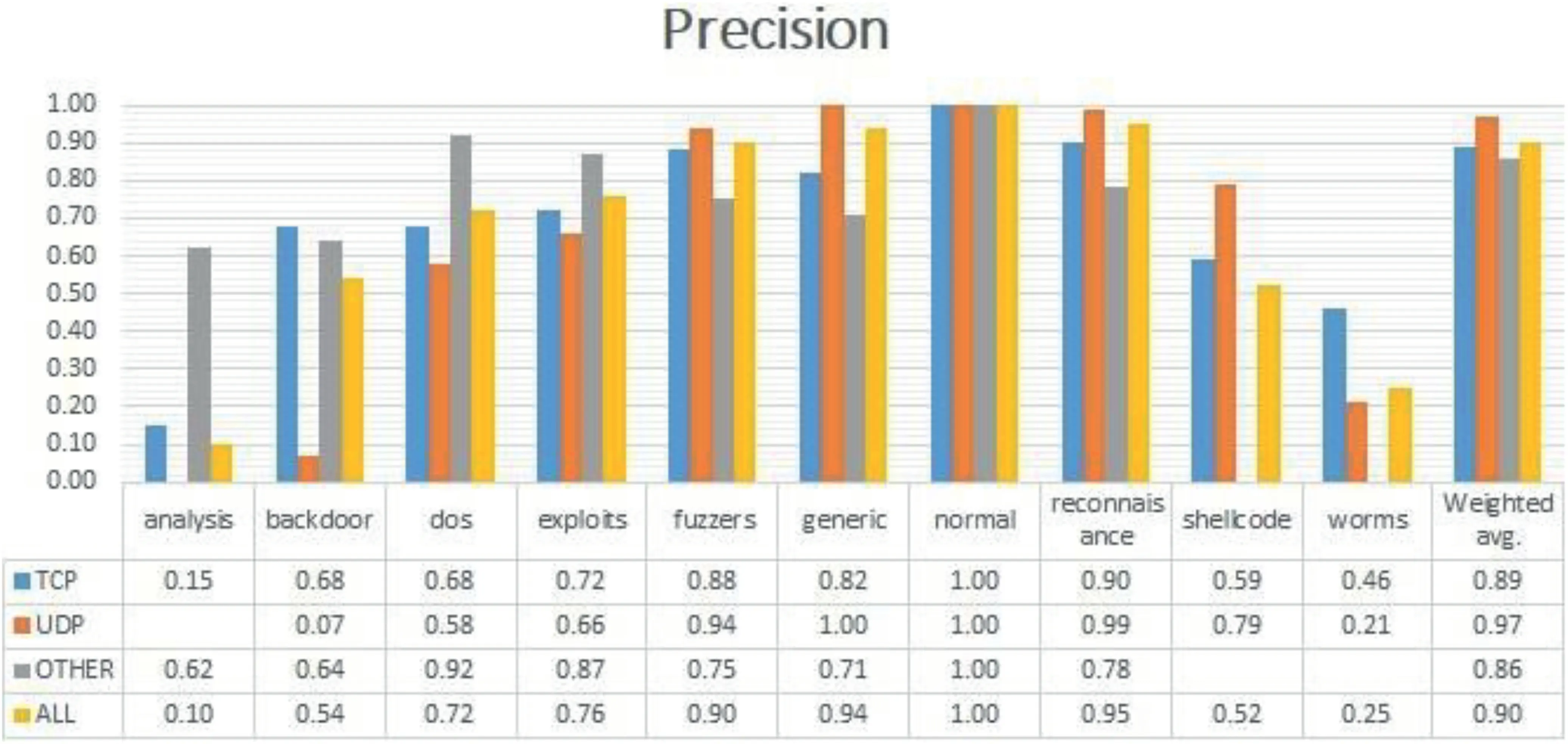
FIGURE 4 Precision comparison

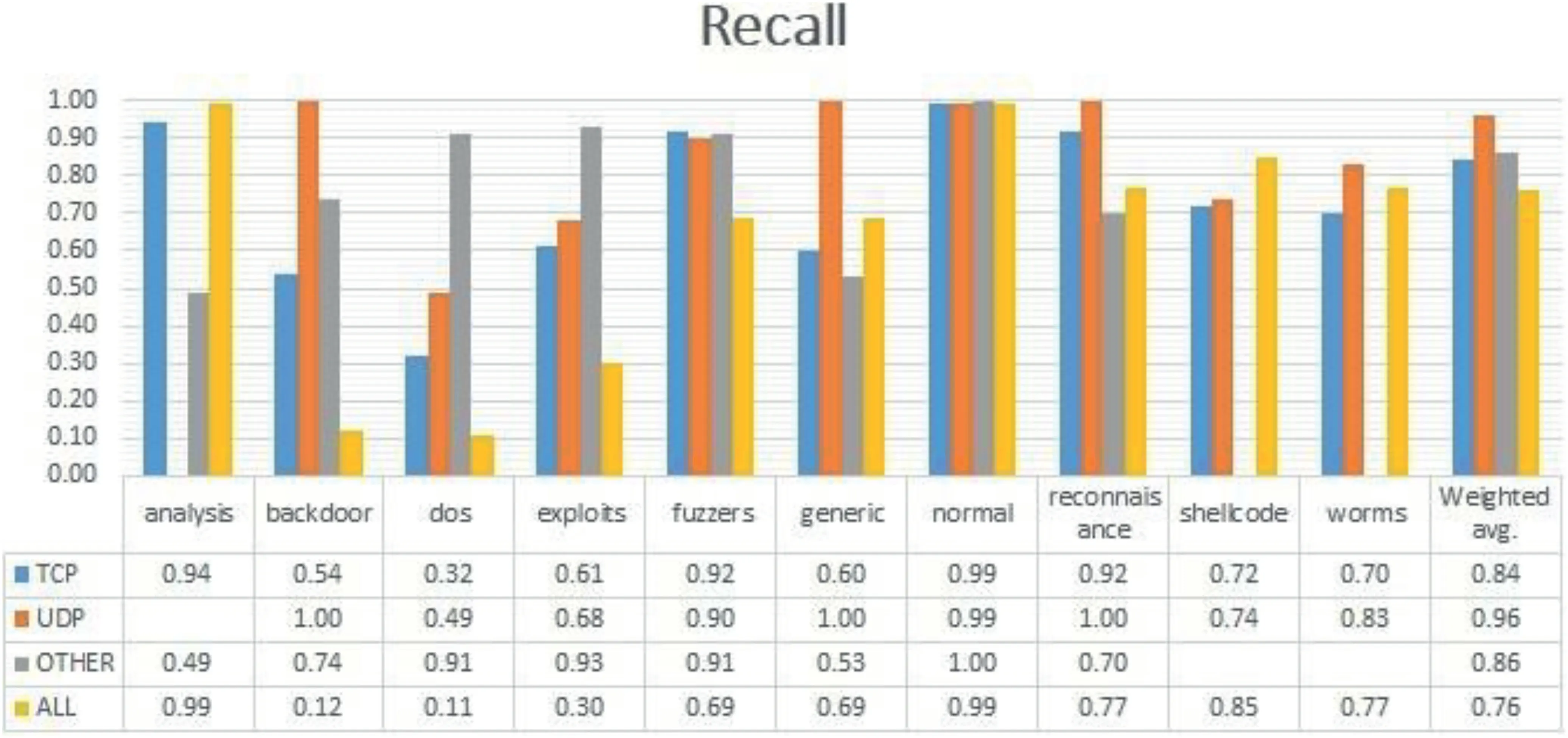
FIGURE 5 Recall comparison

6.2|Discussion

To get insight and relate model's performance with the distribution of data,one way is to visualise the data.There are many visualisation techniques like principal component analysis(PCA),t-distributed stochastic neighbour embedding (t-SNE)etc.In [37,38],the authors used thet-SNE visualisation technique to understand the characteristics of datasets.t-SNE is a non-linear dimensionality reduction technique that turns the high-dimensional feature vector into two or more dimensions[1].We have usedt-SNE to visualise the output of each layer in our model to understand how each layer is behaving.Figure 7a-d represent the output of the model for TCP,Figure 7e-h visualise the output of the model for UDP;similarly,Figure 8a-d and Figure 8e-h visualise outputs of the model for OTHER and ALL,respectively.From feature visualisation in Figures 7,8,we can see that the overlap of classes in TCP,OTHER and ALL data are much more compared to UDP.UDP classes are somehow easily separable compared to the other three categories.That might be one of the reasons that the model is performing better in terms of precision,recall,andf-score on UDP compared to the other data categories.From the comparison of Figures 4,5,6,we can see that the model weighted scores on the UDP data are 0.97 for precision,0.96 for recall,and 0.97 forf-score,which are the highest among all.We also observe that the performance on the ALL category is lower than TCP,UDP,and OTHER in terms off-score measure,which is why we split the data into different protocol categories,as it was mentioned in section 1.

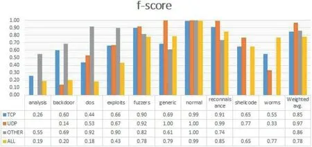
FIGURE 6 f-score comparison

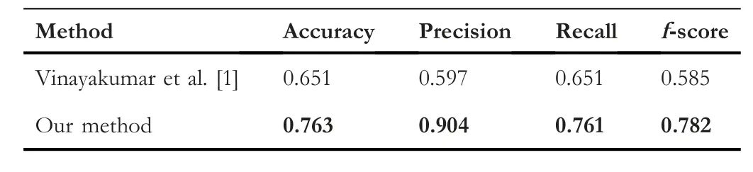
TABLE 9 Overall comparison for multi-classification with different metrics

6.3|Future work

With the rise of ubiquitous ML and DL,malicious actors are also finding new ways to exploit ML/DL.Adversarial attacks are techniques of such malicious acts,which attempt to fool models with deceptive data and lead to misclassification.Ravi et al.[39] proposed a DL-based framework for the DNS data analysis aiming to detect randomly generated DNS and domain names homograph attacks without the requirement for any reverse engineering or using non-existent domain inspection.The authors conducted detailed experiments to evaluate the robustness of their method on benchmarked datasets against threedifferent adversarial attacks:MaskDGA,Charbot,and DeepDGA.The study highlights the need for more robust detection against adversarial learning.The authors in [40]argue that traditional metrics like,for example,accuracy are not sufficient for evaluating security-sensitive ML systems,so they proposed a method named adversarial robustness score (ARS) for quantifying and comparing adversarial threats for IDSs.

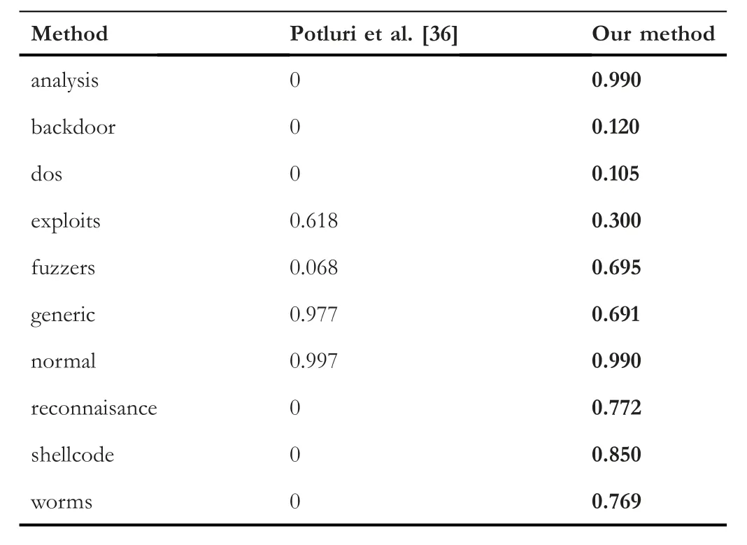
TABLE 10 Class-wise comparison for multi-classification based on accuracy

Here,we propose a future framework to extend our current work with an additional feature to evaluate the robustness of our CNN-based model against adversarial attacks.However,network packets impose more constraints on their features that lead to fewer expose to adversarial attacks compared to an image data,but still,the risk is huge and requires cautious treatment.

The main steps of this framework would be

· First,we are going to identify which features are vulnerable for manipulation,for example,inter-arrival time (IAT) and packet length might be more likely manipulable compared to source and destination ports.We will investigate the importance of these features towards prediction if we can leave them out to avoid the risk.

· Identify commonly used adversarial machine learning(AML) based on the literature and evaluate our model's robustness similar to the work done in[40],except that they tested on RNN and we will test on CNN.However,they used their own metric(ARS),we will compare the goodness of ARS against traditional metrics in our scenario.

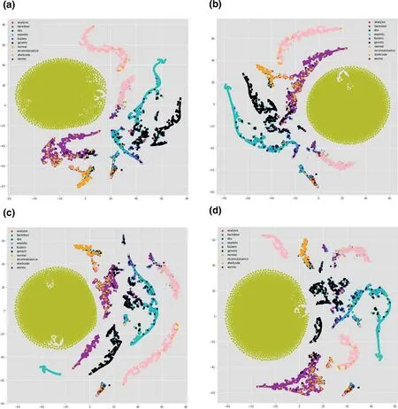
FIGURE 7 t-distributed stochastic neighbour embedding (t-SNE) visualisation of transmission control protocol (TCP) and user datagram protocol(UDP) in 4 layers of convolutional neural network (CNN).(a) t-SNE visualisation of TCP in layer 1;(b) t-SNE visualisation of TCP in layer 2;(c) t-SNE visualisation of TCP in layer 3;(d) t-SNE visualisation of TCP in layer 4;(e) t-SNE visualisation of UDP in layer 1;(f) t-SNE visualisation of UDP in layer 2;(g) t-SNE visualisation of UDP in layer 3;(h) t-SNE visualisation of UDP in layer 4

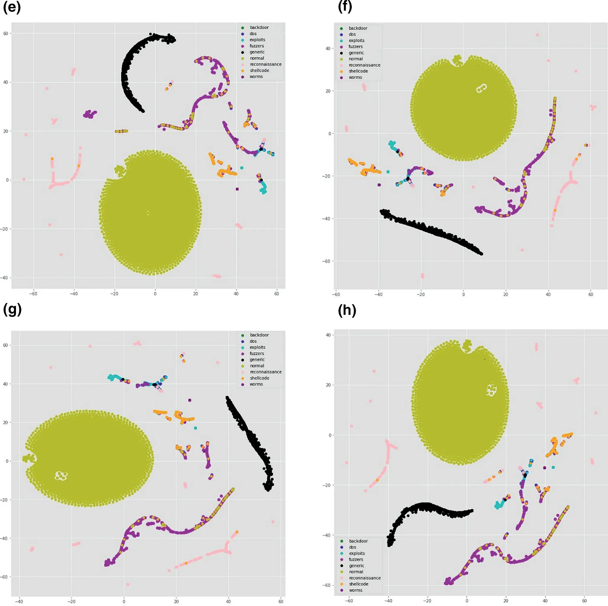
FIGURE 7 (Continued)

· Alternate solution to manipulable feature omission is increasing the robustness of the model against adversarial attacks by augmenting the training set by adversarial attack sample.We will add attack samples and flag them as new attacks and evaluate the model,similar to the work is done in [40],except that we will test on different network architecture and also we will test on a same number of backpropagation as well as on the different number of backpropagation.

· We will evaluate our newly proposed framework on both commonly used datasets that is,UNSW-NB15 and NSLKDD.

7|CONCLUSION AND FUTURE WORK

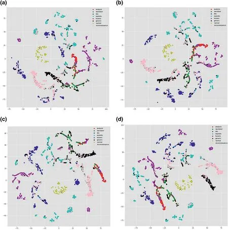
FIGURE 8 t-distributed stochastic neighbour embedding (t-SNE) visualisation of OTHER and ALL in 4 layers of convolutional neural network (CNN).(a)t-SNE visualisation of OTHER in layer 1;(b)t-SNE visualisation of OTHER in layer 2;(c)t-SNE visualisation of OTHER in layer 3;(d)t-SNE visualisation of OTHER in layer 4;(e)t-SNE visualisation of ALL in layer 1;(f)t-SNE visualisation of ALL in layer 2;(g)t-SNE visualisation of ALL in layer 3;(h)t-SNE visualisation of ALL in layer 4

This paper proposes a network anomaly detection using the DL method.We use 1-D CNN architecture to develop a neural network model and incorporate the SMOTE over-sampling method to solve the class-imbalance issue in the dataset.The model was evaluated on the sample of the UNSW-NB15 dataset.The dataset was split into different protocol categories and each category was treated independently.The experimental results show that treating independent categories yield better results in the case of Recall andf-score;however,it is not obvious for the Precision.In this study,we used a sample data and applied only one type of over-sampling technique(SMOTE).In the future studies,we will conduct a comparative study on different sampling techniques and test the model with further hyper tuning and full size of benchmarked datasets.Also,we are going to implement the proposed framework suggested in Section 6.3.

ACKNOWLEDGEMENT

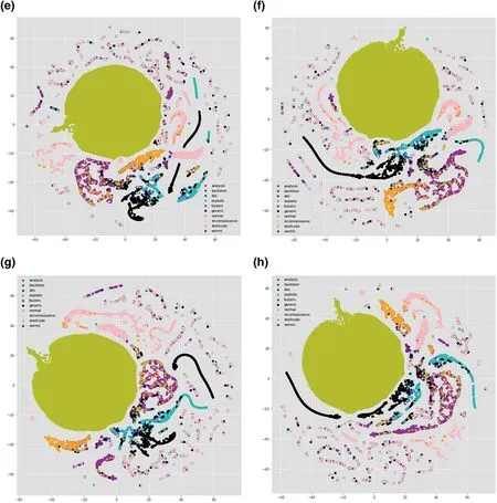
FIGURE 8 (Continued)

None.

CONFLICT OF INTEREST

The authors declare no conflict of interest.

DATA AVAILABILITY STATEMENT

The data has been used in this study is UNSW-NB15,which is freely available for research purposes.

ORCID

Mohammad Kazim Hooshmandhttps://orcid.org/0000-0002-7840-7383