D″ anisotropy inverted from shear wave splitting intensity

Chao Zhang and Zhouchuan Huang

School of Earth Sciences and Engineering, Nanjing University, Nanjing 210023, China

ABSTRACT The D″ layer, located at the bottom of the mantle, is an active thermochemical boundary layer. The upwelling of mantle plumes,as well as possible plate subduction in the D″ layer, could lead to large-scale material transformation and mineral deformation,which could result in significant seismic anisotropy. However, owing to limited observations and immense computational cost,the anisotropic structures and geodynamic mechanisms in the D″ layer remain poorly understood. In this study, we proposed a new inversion method for the seismic anisotropy in the D″ layer quantitatively with shear wave splitting intensities. We first proved the linearity of the splitting intensities under the ray-theory assumption. The synthetic tests showed that, with horizontal axes of symmetry and ray incidences lower than 30° in the D″ layer (typical SKS phase), the anisotropy is well resolved. We applied the method to the measured dataset in Africa and Western Europe, and obtained strong D″ anisotropy in the margins of the large low shear-wave velocity provinces and subducting slabs. The new method makes it possible to obtain D″ anisotropy,which provides essential constraints on the geodynamical processes at the base of the mantle.

Keywords: seismic anisotropy; splitting intensity; D″ layer; plume; slab.

1. Introduction

The D″ layer, located in the lowermost 200 km of the mantle, is an active thermochemical boundary layer above the core-mantle boundary (CMB; Figure 1) (Nakagawa and Tackley, 2008; Lay, 2011). The material transformation and tectonic deformation caused by large-scale geodynamic activities, such as mantle upwelling and plate subduction, cause complex material distribution patterns and structural morphologies (e.g., Lay et al., 2006; Van Der Hilst et al., 2007). For example, the large low shearwave velocity provinces (LLSVPs) that cover large areas beneath Africa and the Pacific are considered to have an important relationship with the deep mantle cycle.Compared to those of the crust and upper mantle, the structural properties and geodynamic modes of deeper areas like the D″ layer remain unclear. A full understanding of the material composition and structural morphology of the D″ layer is essential for understanding deep mantle convection with its dynamic mechanism and may also provide useful information for simulating the thermal reciprocity between the mantle and core (Sumita and Olson, 1999; Gibbons and Gubbins, 2000; Aubert et al., 2008; Gubbins et al., 2011; Wang S and Tkalčić,2021).

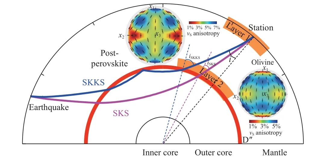
Figure 1. A carton showing the ray paths of SKS and SKKS phases that sample anisotropy in the mantle. i denotes the incidence right beneath the station, iSKS and iSKKS show the incidences of SKS and SKKS in the D′ layer, respectively.Two insets show the mineral anisotropy of the olivine in the upper mantle and the post-perovskite in the D′ layer. The black bar denotes the fast polarization direction. The x1, x2, and x3 axes are respectively north-south, east-west, and vertical directions.

Large-scale tectonic movements accompanied by mineral deformation and material transformation could form macroscopic heterogeneity and anisotropy in an orderly dynamic mode. Seismic anisotropy is an important feature that reflects the deformation and dynamics in the Earth (Crampin, 1985; Savage, 1999; Eberhart-Phillips and Reyners, 2009; Mainprice, 2015; Liu X and Zhao DP,2017). Shear wave splitting is a significant piece of evidence for anisotropy within the Earth (Crampin, 2011;Qaysi et al., 2018) . In an anisotropic medium, the incident shear wave splits into two quasi-shear waves with different propagation speeds and orthogonal polarization directions.Two important parameters are used to reflect the seismic property of the anisotropic medium: time delay between the two quasi-shear waves that reflects the trade-off between the anisotropic strength of the medium and the thickness of the anisotropic layer, and the fast polarization direction that is related to the structure of the anisotropic medium or its internal crystal arrangement (Silver and Savage, 1994 ).

Teleseismic phases, such as SKS and SKKS, are often used to study anisotropy in the Earth (e.g., Niu FL and Perez, 2004; Lynner and Long MD, 2014; Reiss et al.,2019; Figure 1). As P-wave converts to S-wave at the CMB, the anisotropic information from seismic records along the propagation path is restricted to the side beneath the station, and the initial polarization direction of the shear wave before splitting can also be determined by the back azimuth. In addition, the paths of these seismic rays in the upper mantle are nearly vertical (Figure 1). The differentiation of the SKS and SKKS splitting in the same event-station pair can be used to semi-qualitatively compare the difference of anisotropy in different locations of the D″ layer (Lynner and Long MD, 2014; Grund and Ritter, 2019; Lutz et al., 2020; Asplet et al., 2020; Roy et al., 2014; Deng J et al., 2017; Creasy et al., 2020). This splitting analysis could also be applied to S-ScS phase pairs after correcting for the anisotropic contribution from the upper mantle on both the source and receiver sides(Wolf et al., 2019). Direct S-waves can provide additional constraints on anisotropic structures using the reference station technique (Eken and Tilmann, 2014; Confal et al.,2016). However, no unique quantitative estimate of the D″anisotropy has been achieved thus far.

Conventional shear wave splitting analyses include the rotation correlation method (Bowman and Ando, 1987),transverse energy minimization method, or eigenvalue minimization method if the initial polarization of the shear wave is unknown (Silver and Chan, 1991). Chevrot (2000)proposed a more robust multi-channel analysis for shear wave splitting. A new parameter, splitting intensity (IS),was introduced and determined by projecting the transverse component onto the time derivative of the radial component. For an anisotropic medium with a horizontal axis of symmetry, the splitting intensity can be approximated asIS≈-δtsin2β/2, where δtis the time delay and β is the angle between the fast polarization direction and back azimuth. It has the advantages of convenient extraction, high confidence, commutativity, and linear additivity in the presence of multi-layer anisotropic media(Silver and Long MD, 2011). The last two features make it possible to conduct shear wave splitting tomography based on SI measurements, which may quantitatively estimate the layered anisotropy in the Earth.

Several studies also utilized splitting intensity to conduct theoretical inversions for the upper mantle anisotropy (e.g., Favier and Chevrot, 2003; Chevrot, 2006;Long MD et al., 2008; Mondal and Long MD, 2019;Huang ZC and Chevrot, 2021). As the ray paths of the SKS or SKKS phases applied in the inversion are near vertical beneath the station, these tomographic imaging methods use the overlap of finite-frequency kernels along the ray paths to increase the ray crisscross and the robustness of the inversion. Recent works showed that ray theory approximation is suitable for splitting measurement,especially for SK(K)S phases, and matches with results using full-waveform modeling simulation in the simple anisotropic scenarios (e.g., Wolf et al., 2022). In this study,we conducted anisotropic inversion using SI based on ray theory to obtain the seismic anisotropy of the D″ layer and provide important information for constraining deep mantle dynamics.

2. Methodology

Based on previous studies (e.g., Silver and Chan, 1991;Silver and Long MD, 2011), we proved the additivity of splitting intensity through a simple theoretical derivation(see Appendix A). First, we assumed that when the anisotropic media have horizontal axes of symmetry, the change of splitting parameters (i.e., the fast polarization and delay time) with the incident angle and the back azimuth caused by the oblique incidence of seismic wave could be ignored (Figure 1). When a large amount of data is involved in the inversion, the splitting parameters are similar to those when the seismic wave is vertically incident. Second, a layered media model was set to separate the anisotropy in different layers along the ray paths, i.e., the upper mantle and D″ layer (Figure 1).Previous studies have shown that there may be a lateral difference of anisotropic distribution in the D″ layer (e.g.,Lynner and Long MD, 2014; Grund and Ritter, 2019; Lutz et al., 2020; Asplet et al., 2020). Owing to the relatively strong anisotropy in the upper mantle, we adopted a twolayer media model.

The splitting intensity of a single record is the sum of the splitting intensities of the upper mantle and D″ layer(Figure 1). Therefore, the splitting intensity can be expanded, yielding

where δt1, δt2, and φ1,φ2are the time delays and fast polarization directions of the upper mantle and D″ layer,respectively, and θ is the back azimuth of a single record.The above formula can be further organized to obtain

We then apply this parameterization to the whole dataset of splitting intensity measurements, obtaining the following system of linear equations:

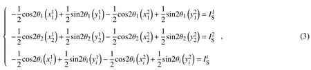
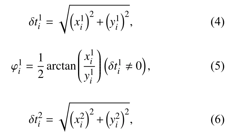
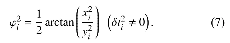
whereiis the record number,(superscripts “1, 2” for the discrimination of the two layers), and the relationships between the unknowns and splitting parameters of the upper mantle and the D″ layer are as follows:

Based on the distribution of the stations and pierce points of the relevant seismic rays at the CMB, the upper mantle and D″ layers were divided into 5° × 5° grids. The two unknown parameters at any coordinate point in the two sets of grids were obtained by the weighted summation of the unknown parameters of the four boundary points on the grid. A simple linear smoothing method was applied to make the splitting parameters of each grid point obtained by the inversion continuous in space. We adopted the LSQR algorithm (Paige and Saunders, 1982) embedded in the CLSQR package to solve the system of linear equations (Equation 3) with an appropriate damping coefficient (1.0 in our inversion).

3. Synthetic tests

Several tests were performed to discuss the feasibility of the inversion algorithm. The model included a two-layer anisotropic structure with horizontal axes of symmetry; the parameters are shown in Table 1. The imaginary rays were constructed by connecting every grid node in the upper layer with those in the lower layer. The synthetic shear wave splitting intensities were calculated using the MSAT Toolkit (Walker and Wookey, 2012). The seismic wave incidences in the upper and lower layers were calculated using the TauP program (Crotwell et al., 1999).

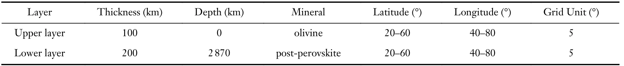
Table 1. Parameters of model setting.

The anisotropic mineral in the upper mantle, i.e.,olivine, has hexagonal symmetry with horizontal axes, and its anisotropic features are consistent for different incidences and azimuths (Figure 1, inset). However, the anisotropy of minerals in the lowermost mantle, such as that of post-perovskite, is complex. A similar hexagonal symmetry with horizontal axes can be assumed only if the seismic waves travel within 30° of the symmetry axis(Figure 1, inset). If the angular differences exceed 30°, no unique symmetry can be assumed. This 30° threshold could also be proven by the analysis of the dipping symmetry axis effects in Chevrot (2000), which is equivalent to the situation in our test of oblique incidence with a horizontal axis of symmetry.

3.1. Test 1: no restriction for the incidence and azimuth

In the first test, we ignored the incident and azimuthal variations of the seismic anisotropy for the postperovskite. The comparisons between the input and inverted splitting parameters for the two layers are shown in Figures 2 and 3. In the upper layer, rays were vertically incident, and the input anisotropies were well resolved in most grid nodes. However, in the lower layer, the input anisotropies were recovered only in the central part of the study region because most of the incidences were subvertical. In contrast, near the periphery, the input model parameters were poorly recovered; the increase in the number of non-vertical rays confuted the assumption of the hexagonal symmetry (Figure 1).

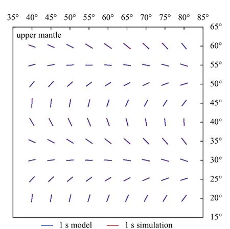
Figure 2. Inverted seismic anisotropy of the upper layer. The blue and red bars represent the input models and inverted results, respectively; the length of the bar denotes the time delay, and its direction is the fast polarization direction.

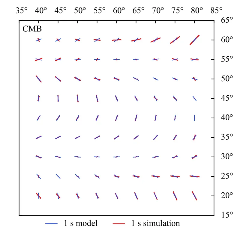
Figure 3. The same as Figure 2 but for inverted seismic anisotropy of the lower layer.

3.2. Test 2: restriction for the incidence

We conducted another test to improve the quality of the simulated inversion of the lower layer. The simulated data were divided into two groups with incident angles at the lower layer less than 30° and greater than 30°according to the anisotropic characteristics of the postperovskite (Figure 1). The new test confirmed that the input anisotropies near the periphery can be well resolved by using the observations with incidences lower than 30°(Figure 4) while they were poorly constrained with the large-incidence data (Figure 5). Moreover, in the above synthetic tests, our models were shown to have uniform thicknesses in each of the two layers, which present identical time delays. As our prior concern in this section was the verification of the assumption of hexagonal symmetry for small-incidence seismic rays in the lower layer, we primarily considered varying the fast polarization directions for convenience and straightforwardness.However, in another synthetic test in the next section, we present more realistic model settings, which contain heterogeneous distributions of both thicknesses and axes of symmetry in each layer.

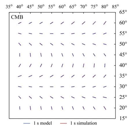
Figure 4. Inverted lower layer anisotropy using rays with incidences ≤ 30°. For the other labeling, see Figure 2.

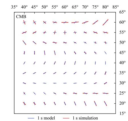
Figure 5. The same as Figure 4 but using rays with incidences ＞ 30°.

3.3. Future work with full-waveform effects

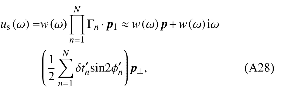
At last, it is necessary to state that our construction of synthetic data focused on the simulation of the splitting process instead of wave propagation throughout the model;therefore, we do not conduct forward full-waveform modeling owing to the huge demands on data volume and computational consumption as well as our primary purpose of anisotropic decomposition. However, moving forward to full-waveform simulation and inversion at the scale of the whole mantle is the indispensable next step of our future work. We substitute the form of splitting intensity fromto those adapted from Favier and Chevrot (2003):

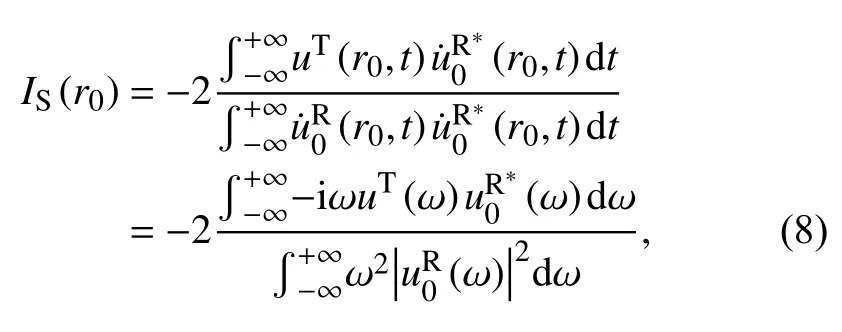
to consider the full-waveform information or finitefrequency effect. Here,uRanduTare the seismograms of the radial and transverse components, ω is frequency (see Chevrot, 2003 for details).

4. Applications

We applied the method to the 1 103 measured shear wave splitting intensities in Europe (Grund and Ritter,2019) and Africa (Reiss et al., 2019). We divided the dataset into two groups. One group contained only the SKS phases with incidences at the CMB within 30°, and the other group contained SKKS phases with corresponding incidences greater than 30° (Figure 6). As shown earlier, the assumption of hexagonal symmetry with horizontal axes in the D″ layer was valid for the SKS phases but not for the SKKS phases. Although inversion using SKKS phases could not be directly linked to the actual anisotropic patterns, they may provide auxiliary information and can be applied in the finite-frequency method, considering varied dipping and incidence effects.

We divided the upper mantle and D″ layer into 5° × 5°grids according to the distribution of stations and seismic ray pierce points at the CMB. Figures 7 and 8 showed the obtained anisotropy in the upper mantle and D″ layers for the SKS and SKKS phases, respectively. Overall, in both sets of inversion results, we obtained stronger anisotropy for the upper mantle than the D″ layer, which was consistent with previous conclusions (e.g., Becker et al.,2012; Reiss et al., 2019).

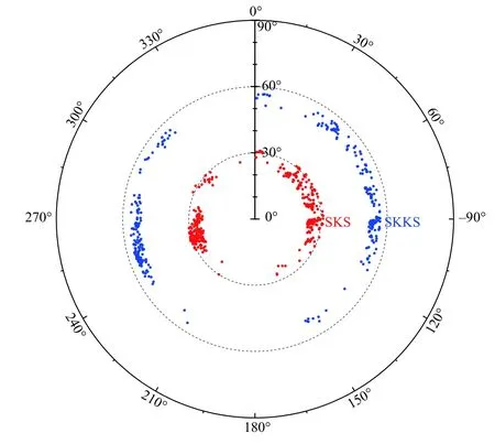
Figure 6. The statistical distribution of azimuths and incidences for ray pierce points at the core-mantle boundary in the dataset. Red and blue points represent the azimuths and incidences of the SKS and SKKS phases, respectively.

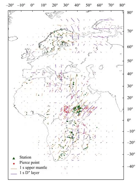
Figure 7. Inversion results using SKS phases. The green triangles indicate the distribution of stations, and the red dots represent the distribution of piercing points at the core-mantle boundary. The orange bar denotes the anisotropy in the upper mantle, the purple bar denotes the anisotropy in the D″ layer.The length and orientation of the short bars denote the time delay and the fast polarization direction, respectively.

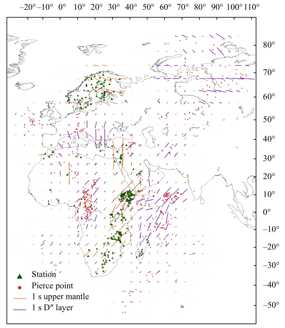
Figure 8. The same as Figure 7 but for the inversion using SKKS phases.

The anisotropies of the upper mantle using the two different datasets were similar, which were consistent with the global SKS splitting compilation (Becker et al., 2012)(Figure 9). To further evaluate the results, we used our inverted anisotropy using SKS phases as input model and conducted the simulated inversion. By defining this model with varying time delays and fast polarization directions,we could assess the inversion quality under more complex conditions (Figures 10 and 11). The results proved that the input models can be well restored.

However, the azimuths of seismic rays in this dataset were confined within a narrow range (Figure 12); thus,the poor intersection of rays would cause some extent of coupling between the parameters of the two layers(Figures 10 and 11). We collected the present research of global SKS splitting measurements and projected the ray segments to pierce points at the D″ layer (Figure 13). The results displayed good azimuthal coverage at the D″ layer under North America, Europe, and North Africa, where direct inversion of the D″ anisotropy was possible. Despite the poor coverage under East Asia, we preferred it as a potential target if the SKS splitting measurements in China were included because these data were not available in the global dataset.

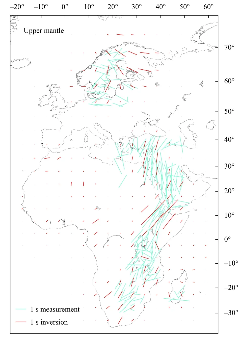
Figure 9. Comparison between the upper-mantle anisotropy obtained in this study (red bars) and the global dataset (cyan bars; Becker et al., 2012). For the other labeling, see Figure 7.

We projected our D″ layer results using SKS phases on the shear wave velocity perturbation using the GyPSuM model (Simmons et al., 2010) (Figure 14). The results beneath Africa were distributed along the boundary of the LLSVP (its rough outline is shown by a prominently red area), which was consistent with previous conclusions on the violent deformation caused by convergence and rise between lowermost mantle plumes and subducting slabs(e.g., Lynner and Long MD, 2014; Reiss et al., 2019;Ritsema et al., 1998). There may be shape-preferred orientation (SPO) in the oriented distribution of molten materials or lattice-preferred orientation (LPO) by the regular arrangement of anisotropic minerals, such as postperovskite (Cottaar and Romanowicz, 2013; Lynner and Long MD, 2014; To et al., 2005). Moreover, the hotter internal materials within the LLSVP were considered isotropic, and the weak anisotropy around the center of LLSVP explained this feature. In the margin of highvelocity region beneath northern Siberia, previous studies have speculated that severe deformation and phase change environment could occur (e.g., Grund and Ritter, 2019).They were caused by horizontal compression and migration of subducting slabs after impinging the CMB,which led to the LPO anisotropy of post-perovskite.

Figure 10. Inverted anisotropy of the upper mantle layer. The cyan and red bars represent the input model and inversion results, respectively. For the other labeling, see Figure 7.

Figure 11. The same as figure 10 but for the D″ anisotropy.

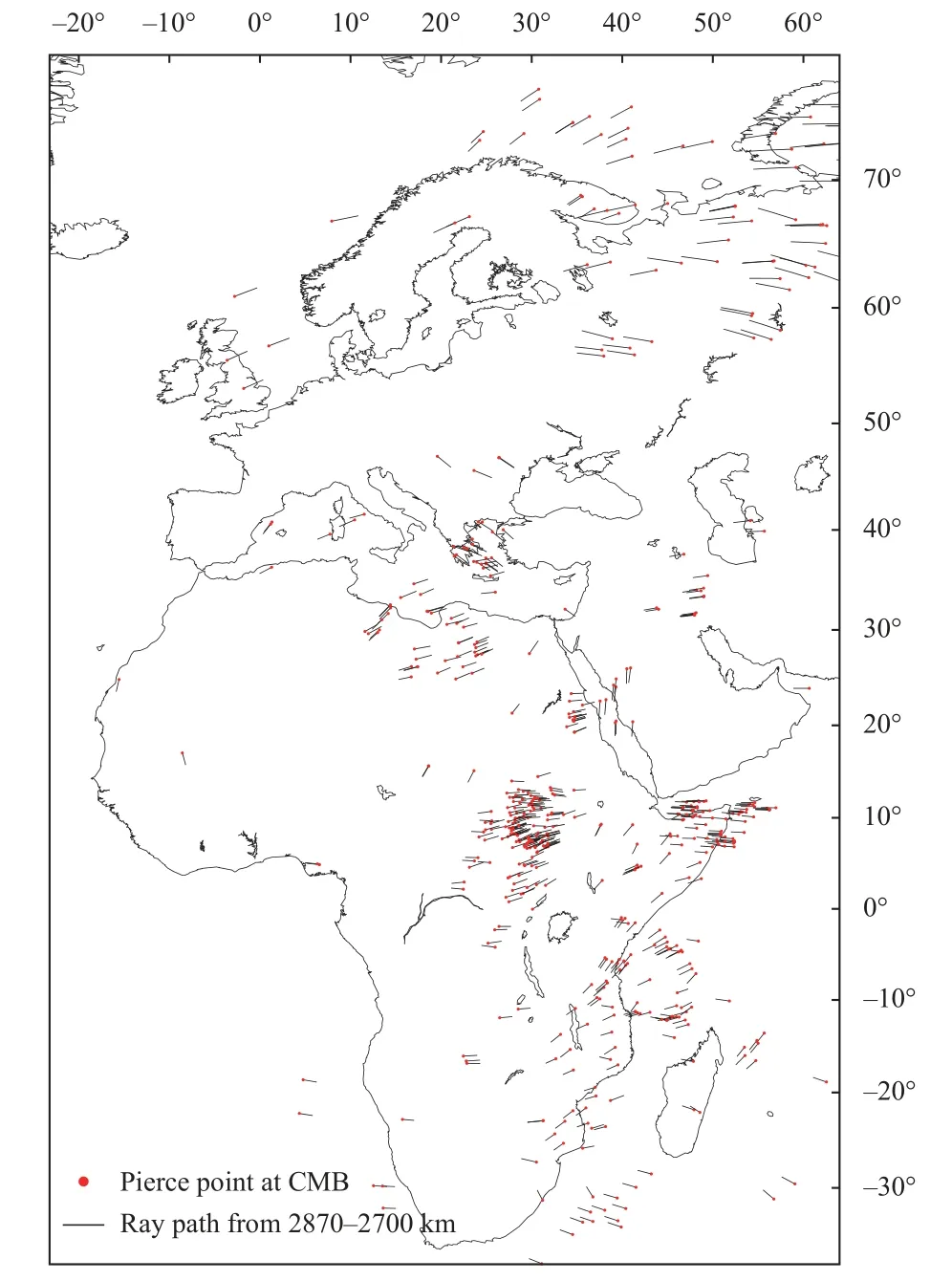
Figure 12. The ray segments of SKS at 2870-2700 km depth.

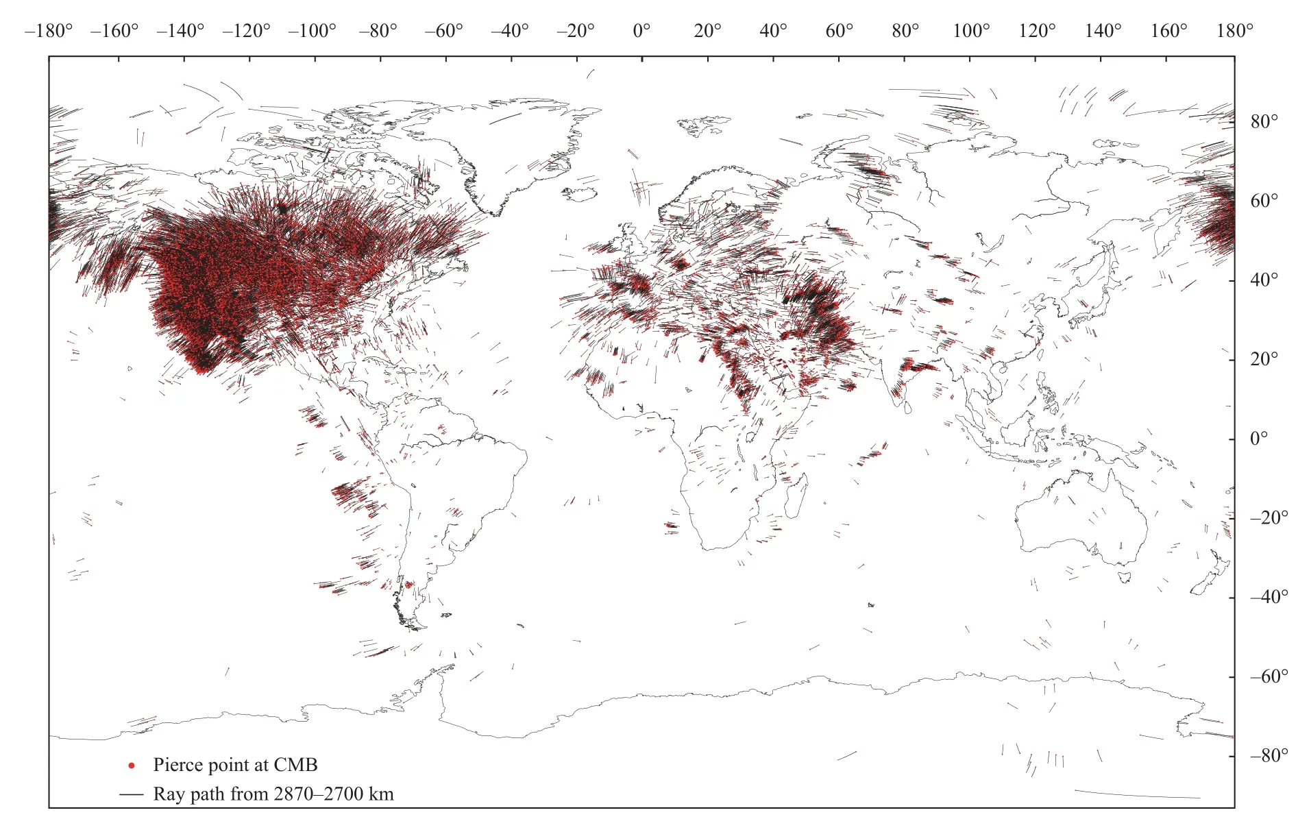
Figure 13. The ray segments of SKS at 2 870-2 700 km depth in the global SKS splitting compilation. Regions with good azimuthal coverage such as North America could be potential study areas to apply the proposed method in this study.

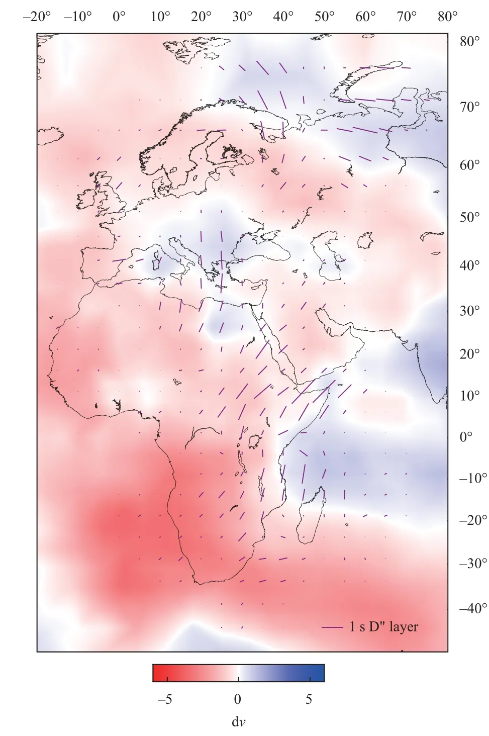
Figure 14. Inverted D″ anisotropy using SKS phases and their comparison with the shear wave velocity at the coremantle boundary. The color scale indicates the deviation of the local shear wave velocity from the average at this depth.

5. Conclusions

We proposed a new inversion method for D″ layer anisotropy based on splitting intensity. In synthetic tests,we found that, for two-layer anisotropic media with horizontal axes of symmetry, reliable anisotropy could be obtained using SKS phases with good azimuthal coverage.In this study, we used the SKS splitting intensity data in Africa and Western Europe to separate the anisotropy of the D″ layer from the contribution of the upper mantle.Our results were consistent with the known or speculated dynamic patterns of LLSVP and subducting slabs above the CMB.

Owing to the limitation of the dataset, the new method can only be used in regions such as North America,Europe, North Africa, and East Asia. The full-waveform information or finite-frequency effect may improve the accurateness and robustness for SK(K)S splitting tomography, which yields more robust inversion for D″anisotropy. The new results further the understanding of the deformation patterns and geodynamics of the D″ layer.

Acknowledgments

This work was supported by the National Natural Science Foundations of China (No. 42174056). We thank the editors and three anonymous reviewers for their constructive comments that improved the manuscript. ZH is also supported by the Deng-Feng Scholar Program of Nanjing University. All the figures were made using GMT(Wessel et al., 2013).

Appendix A: Additivity of splitting intensity

A1. Horizontal axes of symmetry and vertical incidence of waves

A1.1 Single-layer anisotropic medium

Consider the frequency-domain form of a wavelet propagating in an isotropic medium, i.e.,

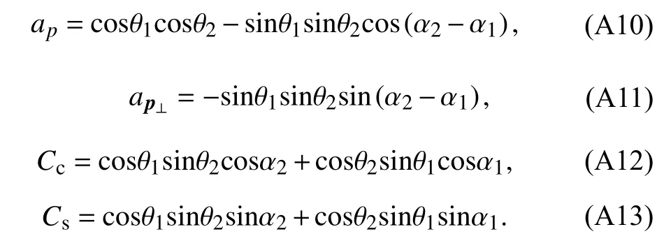
wherepis the unit vector of the initial polarization direction of the wavelet, which corresponds to the back azimuth direction when the wave is vertically incident. The wavelet passing through an anisotropic medium can be realized by multiplying it by a splitting operator :

wherefis the unit vector in the fast polarization direction,andsis the unit vector in the slow polarization direction.The wavelet function after splitting is

where δtis the time delay, and ϕ is the angle between the initial polarization directionpand the fast polarization direction. The radial direction of the surface station is consistent withp, while the transverse direction isp⊥; if θ=ωδt/2 and α=2ϕ, thenus(ω) can be rewritten as follows:

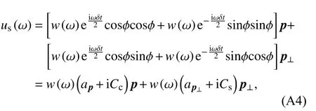
where

A1.2 Two-layer anisotropic media

The process of a shear wave passing through two-layer anisotropic media can be expressed as sequential multiplication of the wavelet by two splitting operators, Γ1and Γ2:

When θ1,2=ωδt1,2/2, α1,2=2ϕ1,2, the definitions of which are the same as before, the subscripts correspond to the splitting parameters of each layer. As the initial polarization direction of the wavelet is consistent with the radial direction of surface stationpfor vertical incidence,we expand the above formula according to (A4) to obtain

A1.3 Multi-layer anisotropic media

When we extend the above process toN-layer anisotropic media, we multiply the wavelet byNsplitting operators in sequence, and also expand according to (A 4),yielding

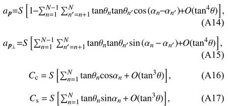
A1.4 Splitting intensity

Assuming that a shear wave passes throughN-layer anisotropic media, the wavelet received by a surface station is

whereKis a complex scalar coefficient; subscriptais the apparent splitting operator, which is implemented toNlayer anisotropic media as equivalent to the splitting operator obtained by a single-layer anisotropic medium;and the corresponding splitting parameters are θaand αa.Then,the splitting operators, the two formulas (A 19) and (A 20)

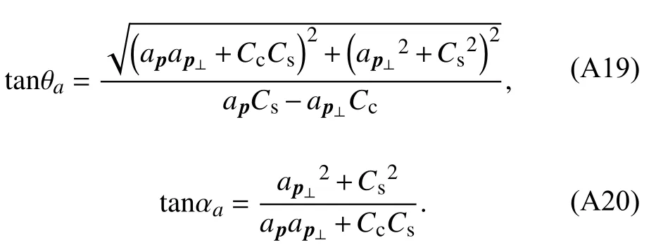
Becauseapandap⊥are formally related to the order of are non-commutative, i.e., they are related to the specific order of anisotropic media layers. Considering the combination of apparent splitting parameters,

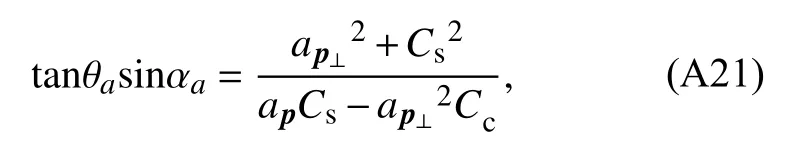
under the low frequency approximation,ap⊥≪ap,ap⊥≪Cs,ap≈1, so that

Equation (A 22) corresponds to the splitting intensity.Obviously, this parameter satisfies commutivity and can be linearly added.

Next, we consider the form of splitting intensity in a single-layer medium:

We then transform the frequency-domain form of Equation (A 23) to the time domain:

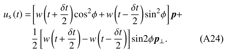
When δtis smaller than the wavelet period, (A 24) can be simplified as

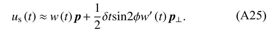
The expression of the splitting intensity in the time domain isIS=δtsin2ϕ/2, which can be obtained by projecting the transverse component of the seismograph onto the time derivative of the radial component.Analogously, in multi-layer anisotropic media,

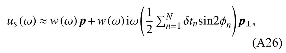
and the corresponding time-domain form is

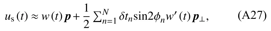
where the splitting intensity isδtnsin2ϕn.Under the assumption that the multi-layer anisotropic media have horizontal axes of symmetry and the wave is vertically incident, the inversion of the splitting parameters by linear equations can be conducted.

A2. Horizontal axes of symmetry and oblique incidence of waves

Now we assume that multiple layers of anisotropic media are distributed in parallel, and that each layer has a horizontal axis of symmetry. When a shear wave passes through these layers at certain angles, the large circular plane of the Earth, where the wave propagation path is located, intersects the plane of each layer. The lines of intersection are parallel to each other, and the directions are the same as the back azimuth direction. As the wave is obliquely incident, the polarization directionpn(subscript‘n’ refers to the nth layer) under isotropic conditions has different angles with each layer. Only when the wave approaches vertical incidence ispnthe same aspdiscussed earlier. When the coordinate system in which the splitting operator Γnacts in each layer of anisotropic media is selected according to the propagation direction of the shear wave,pnis located in the great circular plane of the wave propagation path and is vertical to propagation direction of the wave in the nth layer of the media. Moreover, the direction ofp⊥is always the direction of the transverse component of the station, so that

wherep1is the initial polarization direction when the shear wave passes through the first layer of anisotropic media,pandp⊥are the radial and transverse component directions of the surface station, respectively. The anglebecomes the angle betweenpnand the fast polarization directions in the aforementioned accompanying coordinate system, andis the corresponding time delay, which are both related to the incident angle of the nth layer and the back azimuth.If all the above variables are considered, then the actual shear-wave splitting data are hardly sufficient, with inadequate back azimuth coverage. Therefore, we need to consider the hypothetical simplification.