Dynamical Model to Optimize Student’s Academic Performance

Evren Hincal and Amna Hashim Alzadjali

Department of Mathematics,Near East University,Mersin,10 KKTC,Cyprus

ABSTRACT Excellent student’s academic performance is the uppermost priority and goal of educators and facilitators.The dubious marginal rate between admission and graduation rates unveils the rates of dropout and withdrawal from school.To improve the academic performance of students,we optimize the performance indices to the dynamics describing the academic performance in the form of nonlinear system ODE.We established the uniform boundedness of the model and the existence and uniqueness result.The independence and interdependence equilibria were found to be locally and globally asymptotically stable.The optimal control analysis was carried out,and lastly,numerical simulation was run to visualize the impact of the performance index in optimizing academic performance.

KEYWORDS Academic performance;optimal control;uniform boundedness;Pontryagin Maximum Principle(PMP);existence and uniqueness;stability

1 Introduction

The human capital theory perceives education and learning activities as an investment in people to increase the productivity of goods and services[1].The industrial and technological development of a country depends on literacy as a requirement for its success.This is especially when a literate member of society engages in an active and effective role in the development process.There is no doubt that combining the skills of improving income generation with knowledge of sustainable development assist mankind in improving his material condition of living through the use of resources available to him.

The academic performance of a student serves as the bedrock for knowledge acquisition and the development of skills that directly impact the socio-economic development of a country[2].It determines the success or failure of any academic institution[3].

There are many factors that enhance and impede students’academic performance attributed to students,parents,teachers and environments.The student’s factors include self-motivation,interest in a subject,punctuality in class,regular studying and access to learning materials.Class attendance and students’attitudes toward their learning have an impact on academic performance.In[4],it is confirmed that in the case of mathematics,students’attitude towards the subject has a direct impact on their academic performance.

Qualified teachers and facilitators render effective facilitation which enhances academic performance.However,performance target,completion of syllabus,paying attention to weak students,assignment and student evaluation have significant impact too[5].

Parental background and status have significant impact on student’s academic performance.Educated parent provide home school tutorial to their ward and are more encouraging as well.In[6],it was shown that,students with high level of parental involvement in their academics excel their counterparts with no such involvement.

Environmental factors that inf luence academic performance are enabling environment,infrastructure,adequate facilities and learning materials,well-equipped laboratories,etc.In[7],it is revealed that the availability of physical resources such as the library,textbooks,adequacy of classroom and spacious playing ground affect the performance of the students.Reference[8]emphasized that the use of instructional equipment facilitates effective service delivery and enhances teaching and learning.Distanced school also affects students’performance in the sence that the more school distance,the more tired students become[9,10].

Also,fairly disciplined schools perform better than less or no disciplined schools.Effective discipline is used to control students’behavior,which has a direct impact on their academic performance[11].Furthermore,the student-to-teacher ratio or class size also affects performance.Effective teaching in a moderate class ratio enhances performance[12].

Age has a significant impact on academic performance;older students are likely to drop out than younger ones.Reference[10]showed a significant positive impact of age on academic performance in mathematics and science but the degree of the association is weak.

Mathematical models play a significant role in solving real-life problems[13–15].Moreover,a mathematical model is an important tool used to optimize a real-life problem for the quickest and effective resolution[16–20].In this paper,we study the uppermost priority and goal of educators and facilitators.The dubious marginal rate between admission and graduation rates unveils the rates of dropout and withdrawal from school.To improve the academic performance of students,we optimize the performance indices to the dynamics describing the academic performance in the form of nonlinear ODE.

The paper is arranged as follows:Introduction is given in chapter one,followed by definitions of terms and important theorems in Chapter two.Chapter three gives the detail of model formulation while Chapter four gives stability analysis of the solutions of the model.Chapter five is the detailed formation of optimal control and numerical simulations.

2 Definition and Theorems

Def inition 1:[21](Optimal Control)

A fairly general continuous time optimal control problem can be defined as follows:

Problem i:To find the control vector trajectoryminimize the performance index:

subject to:

where

x=(x1,x2,x3,...,x n)T,f=(f1,f2,f3,...,f n)Tandis a terminal cost function.

Problem ii:Findtfandu(t)to minimize:

subject to:

This special type of optimal control problem is called the minimum time problem.

Def inition 2:[21](Hamiltonian)

With a time varying Largrange’s multiplier function,also known as the co-state define Hamiltonian functionHas:

such that

Theorem 1:[22](Banach’s Fixed Point Theorem)

Let(X,d)be a complete metric space and letT:X→Xbe contractive operator,i.e.,there is a constantα∈(0,1)such that

then there exists a unique fixed pointx∈Xsuch thatTx=x.

The above theorem states the conditions sufficient for the existence and uniqueness of a fixed point,which we will see in a point that is mapped to itself.

Theorem 2:[23](Lyapunov Function Theorem)

Theorem 3:[24](Pontryagin Maximum Principle)

and such that at terminal timetfthe conditions:

If the functionsλ(t),x(t),u(t)satisfy the relation(8),(9)(i.e.,x(t),u(t)are Portryagin extremals),then the condition,

This theorem is used in optimal control theory to find the best possible control for taking a dynamical system from one state to another,especially in the presence of constraints for the state or input controls.

Remark 1:[25]For a minimum,it is necessary for the stationary(optimality)condition to give:

3 Model Formulation

The model is constructed based on the assumption that the new intake is admitted into the average class at the rateλ.The average student A may then become weak,excellent or graduate at the ratesφ,βandθ2,respectively.Below average student B may become weak,average or graduate at the ratesγ,αandθ1,respectively.Excellent student E graduate at rateθ3.But upon mingling with weak student W,the excellent student E may be influenced to become weak at the rateη.The rate at which student leaves school either through death or expelled is assumed to be the same in all the compartments.The schematic diagram of the model is given in Fig.1.

Figure 1:Schematic diagram describing the dynamics of student academic performance

The performance dynamics is described by the nonlinear system of ODE

3.1 Uniform Boundedness

Theorem 4:All the solutions of model are confined within bounded subset

Proof

Let the population size be

then

Solving the linear ODE(17)gives

The long-term behavior of(18)yield

Meanwhile,as time increases without bound all the solutions converge to the equilibrium,of(18),hence the equilibrium is globally asymptotically stable.

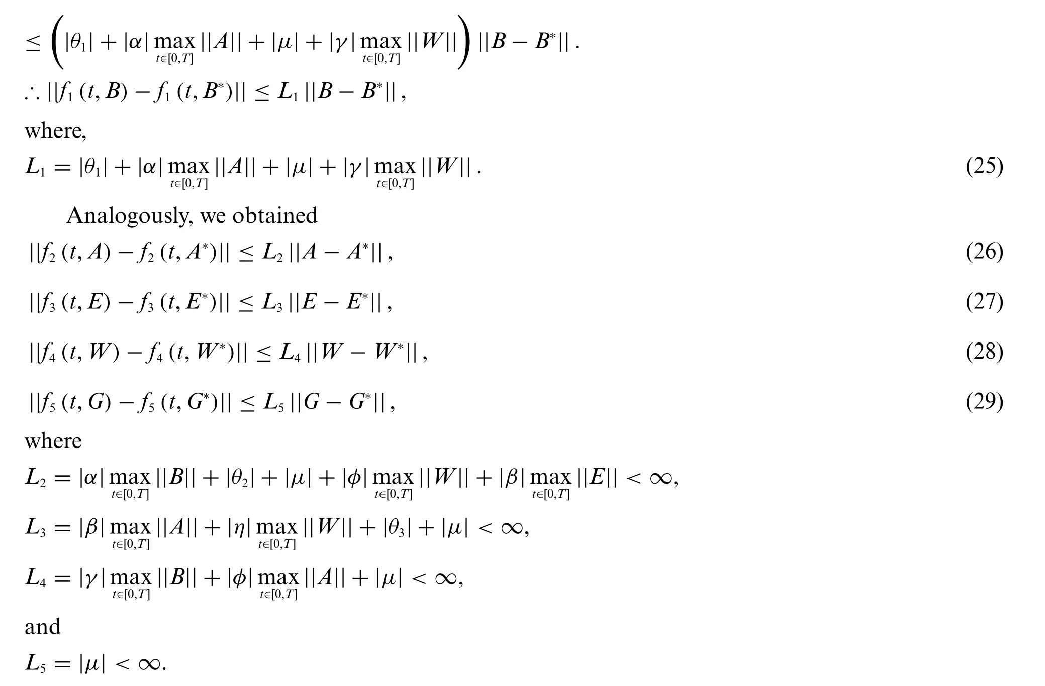
3.2 Existence and Uniqueness

Theorem 5:The system(11)–(15)is Lipschitz continuous

Proof

Let the system(11)–(15)be of the form

4 Stability Analysis

Since the state Eq.(15)depends on the previous states,it suffices to analyze(11)–(15).

4.1 Equilibrium Solution

The system(11)–(15)has the following equilibrium solutions

4.2 Local Stability

From system(11)–(15)we formulate the following Jacobian matrix,and then we test the equilibrium solution in the Jacobian matrix,if all the eigenvalues are negative,then the solution is locally stable,otherwise it is unstable[26,27].

Theorem 7:The independence equilibrium(E0)is locally asymptotically stable.

Proof

The eigenvalues ofJE*are

4.3 Global Stability

Theorem 8:The independence equilibriumE*is globally asymptotically stable in the interior ofΨ.

Proof

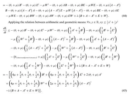
HenceE**is globally asymptotically stable.

5 Formation of Optimal Control

The optimal control strategy is aimed at optimizing student’s academic performance which ref lects in the increase of number of graduating students.

Let the control rates:

u1(t)∈[0,u1(t)max]be the self-motivation that makes weak student to become below average student.

u2(t)∈[0,u2(t)max]be punctuality in class that makes weak student to become average.

u3(t)∈[0,u3(t)max]be the interest in the subject that makes below average student to become average.

u4(t)∈[0,u4(t)max]be regular studying that makes average student to become excellent.

u5(t)∈[0,u5(t)max]be examination performance and character that make below average,average and excellent students to graduate.

Then the control dynamics is described by the nonlinear system of ODE below:

subject to the objective functional;

whereci≥0,i=1,2,...,10 are the weights parameters that balanced the size of the terms.

We seek for optimal controlu*such that

J(u*)=min{J(u):u∈U},

where

Uis the set of admissible controls defined by:

U={ui(t):0≤ui(t)≤1,i=1,2,...10,ui(t)is Lebesguemeasurable}.

5.1 Characterization of Optimal Control

To derive the optimal academic performance of student,define Hamiltonian,

Theorem 10:Letx=(B,A,E,W,G)with associated optimal control varialesu1,u2,u3,u4,u5then there exist a co-state variable satisfying,

Proof

Applying(10),

Analogously,

subject to transversality condition as in[28,29]

Applying the optimality conditionimplies that

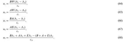
Hence,

6 Numerical Simulation

In this section numerical examples are given to support the analytic results.We use the following values of variables and parameters for the simulations.Fig.2 compares the dynamics of different populations involved in the model.Figs.3 and 4 compare the dynamics of the Weak student to the dynamics of Graduating student and then to the dynamics of Excellent students,respectively.Figs.5–9 show the significance of the control on different populations involved in the model.

A(0)=1000,B(0)=5000,E(0)=50,W(0)=2000,G(0)=5000,

α=0.71,β=0.3,γ=0.51,θ1=0.15,θ2=0.25,θ3=0.6,μ=0.7,λ=0.7,φ=0.55,η=0.2.

Fig.2 depicts the dynamics of all the populations involved in the model.It can be seen that as only Graduate and Weak students reach and pass the fifth year indicating graduation and spillovers,respectively.

Figure 2:Dynamics of different populations in the model

Fig.3 compares the dynamics of Graduate and Weak students.It can be seen that although both reach the fifth year,but Weak students’population didn’t reach zero in the fifth year.This gives the possibility of spillovers.Also,since the population of Weak students is higher than that of Graduate students,there is need for taking appropriate measures to improve students learning.

Figure 3:Comparison between dynamics of weak and graduate students

Fig.4 compares the dynamics of Weak and Excellent students.Clearly the population of Weak students is higher.This is so true in most of our universities and colleges,excellent students have smallest population.

Figure 4:Comparison between dynamics of weak and excellent students

Fig.5 compares the dynamics of Weak students with and without control.The effect of control is clearly seen.It is clear that,when appropriate control measures are taken,students’performances can be improved and the number of graduate students can be increased.

Figure 5:Comparison between dynamics of Weak students with and without control

Fig.6 compares the dynamics of Excellent students with and without control.The effect of control is clearly seen.It is clear that,when appropriate control measures are taken,Population of the Excellent students will be increased.

Figure 6:Comparison between dynamics of excellent students with and without control

Fig.7 compares the dynamics of Average students with and without control.The effect of control is clearly seen.It is clear that,when appropriate control measures are taken,Population of the Average students will be increased.

Fig.8 compares the dynamics of Below-Average students with and without control.The effect of control is clearly seen.It is clear that,when appropriate control measures are taken,the performance of Below Average students will be improved.

Fig.9 compares the dynamics of Graduate students with and without control.The effect of control is clearly seen.It is clear that,when appropriate control measures are taken,the overall population of Graduate students will be increased.This is the ultimate target.

Figure 7:Comparison between dynamics of average students with and without control

Figure 8:Comparison between dynamics of below average students with and without control

Figure 9:Comparison between dynamics of graduating students with and without control

7 Conclusion

To improve the academic performance of students,we optimize the performance indices to the dynamics describing the academic performance in the form of nonlinear system ODE.We established the uniform boundedness of the model and the existence and uniqueness result.The independence and interdependence equilibria were found to be locally and globally asymptotically stable.The optimal control analysis was carried out,and lastly,numerical simulation was run to visualize the impact of the performance index in optimizing academic performance.

From the numerical simulation result,it can be observed that the weak students’population dominates other populations.This shows that when there is too much intermingling between Weak students and the other categories of students,it will be to the disadvantage of the other students.

The significance of the optimal control is also clearly shown.There is a drastic increase in the populations of Average,below–Average,Excellent and Graduating students’population after the application of the control.On the other hand,there is a drastic decrease in the population of weak students after the application of the control.

In the future,the fractional analogue of the model should be considered and real data should be used to validate it.

Funding Statement:The authors received no specific funding for this study.

Conflicts of Interest:The authors declare that they have no conf licts of interest to report regarding the present study.