Joint Model of Wind Speed and Corresponding Direction Based on Wind Rose for Wind Energy Exploitation

YANG Zihao, LIN Yifan, and DONG Sheng, *

Joint Model of Wind Speed and Corresponding Direction Based on Wind Rose for Wind Energy Exploitation

YANG Zihao1), LIN Yifan2), and DONG Sheng1), *

1) College of Engineering, Ocean University of China, Qingdao 266100, China 2) Huadian Heavy Industries Co., Ltd., Beijing 100070, China

As a common and extensive datum to analyze wind, wind rose is one of the most important components of the meteorological elements. In this study, a model is proposed to establish the joint probability distribution of wind speed and direction using grouped data of wind rose. On the basis of the model, an algorithm is presented to generate pseudorandom numbers of wind speed and paired direction data. Afterward, the proposed model and algorithm are applied to two weather stations located in the Liaodong Gulf. With the models built for the two cases, a novel graph representing the continuous joint probability distribution of wind speed and direction is plotted, showing a strong correlation to the corresponding wind rose. Moreover, the joint probability distributions are utilized to evaluate wind energy potential successfully. In cooperation with Monte Carlo simulation, the model can approximately predict annual directional extreme wind speed under different return periods under the condition that the wind rose can represent the meteorological characters of the wind field well. The model is beneficial to design and install wind turbines.

angular-linear distribution; wind speed; wind direction; wind rose; wind energy; Monte Carlo simulation

1 Introduction

As a strategic emerging industry, wind power has been growing rapidly and is being utilized worldwide due to the clean nature of wind energy (Alsaad, 2013; Han., 2019). As pointed by Wang. (2016) and Koeppl (1982), the distribution of wind speed can be used to evaluate the mean available wind energy, irregularity factor, and recoverable power or power factor for a given type of wind turbine (Huang and Wan, 2012; Masseran., 2012; Pishgar-Komlesh., 2015). Given that wind speed is naturally related to its direction, research on wind characteristics based on bivariate statistical models representing wind speed and direction can become more accurate for the evaluation of wind resources, thereby benefiting the design and implementation of a more efficient system for harnessing wind energy (Ovgor., 2012; Stephen., 2013). However, the current common method considers the distribution of wind direction roughly by the wind rose (Keyhani., 2010; Mirhosseini., 2011; Tiang and Ishak, 2012).

Therefore, obtaining the joint probability distribution of wind speed and direction and applying it to generate pseudorandom numbers can be useful in exploring wind resources (Vanem., 2020). As pointed by Li. (2013) and Wang. (2015), when the wind speed exceeds 25ms−1, it is prone to exhibiting abnormal wind turbulence and shear, which can cause a fatal blow to wind turbines. Meanwhile, the increased loads on blades and towers may meet or exceed their corresponding design loads, which can induce blade fracture and even wind towercollapse. Through the generated pseudorandom numbers, on the one hand, the simulative data can help analyze the reliability of structures under wind loads, especially for structures that are unsymmetrical in space (, offshore wind turbines), whereas current structural designs usually only consider the distribution of wind speed or the wind speed distribution in specified directions; on the other hand, it can be used to predict the directional property of extreme wind conditions by Monte Carlo simulation.

As a typical angular-linear distribution, the joint distribution of wind speed and direction has been extensively investigated by many experts and scholars on the approach of model building. However, a large part of the models proposed has a discrete marginal distribution of wind direction, and literature about building the smooth joint distribution of wind speed and direction is scarce. McWil- liams. (1979) and McWilliams and Sprevak (1980) proposed an isotropic Gaussian model based on the assumption that the longitudinal component of wind is independent of the component that is orthogonal to it. Weber (1991, 1997) canceled the restriction in which the standard deviations of the longitudinal and lateral are equal, proposed a more general anisotropic Gaussian model. Moreover, on the basis of the principle of maximum entropy, a method to obtain angular-linear distribution was proposed by Johnson and Wehrly (1978); this method attracted considerable attention for its clear form and applicability. The probability density function (PDF) of the model is composed of the marginal distributions of wind speed, wind direction, and their circular correlation variable. Carta. (2008b) constructed this model with a singly truncated from below the Normal-Weibull mixture distribution for marginal distribution of wind speed, and a finite mixture of von Mises distributions for marginal distribution of circular variable including wind direction and joint variable. Then, they utilized the model to analyze data of several weather stations in Spain’s Canary Islands and compared it with the isotropic and anisotropic Gaussian models, which show good performance. Erdem and Shi (2011) compared this kind of angular-linear distribution with bivariate distributions based on Farlie-Gumbel-Morgenstern copula and anisotropic lognormal approaches.Qin. (2010) used the generalization distribution of von Mises to fit the distribution of the joint variable of wind speed and direction. Compared with the existing model, the result shows that the new model can provide a high degree of fitness for wind data. Schindler and Jung (2018) utilized mixed Burr-generalized extreme value distribution and Gaussian copulas to construct a joint distribution for the estimation of directional wind energy. Cook (2019) proposed the OEN mixture model for fitting the joint distribution of wind speed and direction and utilized it at 128 stations. The results implied that the model has global potential in modeling the joint and marginal distribution of wind speed and direction. Furthermore, on the basis of the copula function, a novel approach was presented by Li. (2019) to model the joint cumulative distribution function (CDF) of wind speed and direction for a wind-resistant design of engineering structures. In addition, an effective and practical way to predict extreme wind speed under a certain return period was provided. Ye. (2019) introduced a finite mixture distribution, including mixture Weibull distributions and von Mises distributions, to model the joint distribution of wind speed and direction. To construct the model, an extended parameter estimation algorithm was proposed. As for the nonparametric approach to construct the joint distribution of wind speed and direction, Zhang. (2013) developed a smooth multivariate wind distribution model to capture the coupled variation of wind speed, wind direction, and air density. Han. (2018) proposed two nonparametric models, namely, the nonparametric kernel density and nonparametric JW models, to model the joint probabilistic distribution of wind speed and direction; the performance of these models are more robust than that of parametric models.

The joint distribution of wind speed and direction is usually established at target areas under a condition wherein adequate weather data can be acquired; thus, the observing equipment must fit certain requirements and restrict its range of applicability. As a common and extensive datum to analyze wind characteristics, the wind rose is simple and intuitive to show the rough distribution of wind speed and direction. However, in practical applications, an error occurs if 16 wind speed distributions corresponding to the different directions are used to characterize the entire wind farm’s meteorological characteristics of wind. If the joint distribution of wind speed and direction can be built by wind rose, then it would greatly relax the requirements of data used in joint model building and remarkably improve the accuracy of the wind meteorological element analysis. Especially for wind farms that lack meteorological data, this method can be beneficial.

This paper is organized as follows: Section 2 introduces the lower-truncated distribution proposed for wind speed, the commonly used wind direction distribution, and the angular-linear model with their parameters’ estimation me- thods. Furthermore, several evaluation criteria are listed for testing the goodness of fit. In the same section, we propose the algorithm of pseudorandom number generation and how to estimate extreme wind speed. In Section 3, the model is applied in two wind roses collected from the Changxingdao and Lüshun weather stations for wind energy assessment and directional extreme wind speed estimation. The conclusions of this study are summarized in Section 4.

2 Methodology

2.1 Lower-Truncated Distribution for Wind Speed

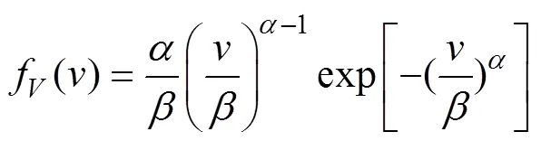
The distribution of wind speed widely used in ocean engineering design and wind energy exploitation is usually skewed. Many studies have been published in the scientific literature related to the theoretically skewed distribution of wind speed. Carta. (2009) summarized the PDFs used to describe the distribution of wind speed, from which the Weibull, Rayleigh and truncated normal from below distributions are selected as candidates in modeling wind speed and are listed as follows.

The PDF of Weibull distribution is

where≥0, and,>0 are shape and scale parameters, respectively.

The PDF of Rayleigh distribution is

where≥0 and>0 are scale parameters of the function.

The PDF of the truncated normal from below distribution is

where≥0, andandare the mean value and standard deviation of the normal distribution, respectively.

However, wind roses drew by the Beaufort scale generally do not include the direction distribution of calm, which is called zero-order wind with speed not exceeding 0.3ms−1. For the zone where the frequency of clam () constitutes a considerable proportion and the wind frequency of prevailing directions takes alargeproportion, ifis treated as uniformly distributed in all directions, then the constructed model obtains a subjective error. To avoid this problem, directional wind () must be defined as the wind with speed above 0.3ms−1.

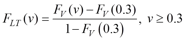
Truncated distribution, which is applied widely in the wind characteristic description, is suitable for conditions where the variable is confined to a certain range. Kantar and Usta (2015) first utilized upper truncated Weibull distribution to model wind speed and estimate wind power density. The results showed that it outperforms the well-known Weibull distribution. Hence, to model the speed of, a novel kind of lower-truncated distribution was proposed by setting the lower truncation point as 0.3. The PDF and CDF of such distribution are given by Eqs. (4) and (5).

Overall, the applicability of single theoretical wind speed distribution varies with data. On this basis, it is a trend to use mixed distributions to model wind speed (Jaramillo and Borja, 2004; Carta and Ramírez, 2007a, 2007b; Akdağ., 2010; Allouhi., 2017; Mazzeo., 2018). In this study, mixed distributions of lower truncated Wei- bull-lower-truncated Rayleigh (MLTWR) and lower-truncated Weibull-lower-truncated truncated normal from below (MLTWTN) together with single distributions, including lower-truncated Weibull (LTW) and lower-truncated Rayleigh (LTR), are selected as the alternative models for wind speed. The form of mixed distribution is given by

wheref1() andf2() are two components, which could be any kind of lower-truncated distribution; 0<0<1 is the weight off1().

2.2 Wind Direction Distribution

A finite mixture of von Mises distributions has been proven to be a flexible model for angular variables (Carta., 2008a, 2008b; Qin., 2010; Erdem and Shi, 2011; Masseran., 2013). Its PDF is listed in Eq. (7).

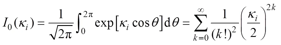
whereÎ[0, 2π),w>0 is the non-negative weight parameter adding up to one; 0≤μ≤2π andκ>0 are the mean value parameter and concentration parameter, respectively. Here,0(κ) is the zeroth modified Bessel function of the first kind, expressed as

2.3 Angular-Linear Distribution

The PDF for angular-linear distribution defined by John- son and Wehrly (1978) is

wheref() andΘ() are the PDFs of wind speed and direction, respectively;(•) is the PDF of the angular variable, expressed as

whereF() andΘ() are CDFs of wind speed and direction, respectively.

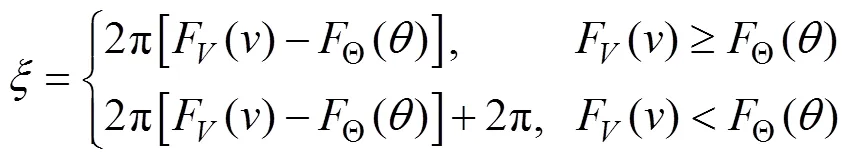
LetΘ() be the CDF of’s direction; then, the circular variableofis defined as

Hence, the joint PDF ofis given by

where(•) is the PDF of, andΘ() is the PDF of’s direction. Whenequals zero, Eq. (12) returns to the original function Eq. (9).

2.4 Model of Joint Variable ψ

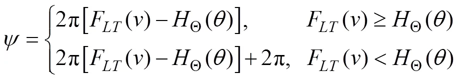
According to Eq. (12), the core of constructing the joint distribution is to obtain the PDF of the joint variable. Carta. (2008a) pointed that in case analysis, a mixture of twovon Mises distributions can provide enough precision in modeling joint variables. The conclusion was reanalyzedon the basis of the definition of joint variablein Eq. (11);is dividedinto

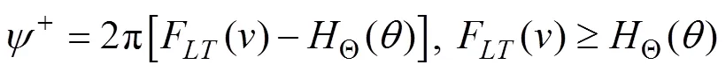
The probability that the joint variableequals to a random number0is

Assume the PDFs of+and–are von Mises distributions1(;1,1) and2(;2,2), and the probability(Î+) and(Î+) adding up to one are1and2, respectively. Then, the PDF ofcan be given by

Although the form of Eq. (15) is the same as that mentioned previously (Carta., 2008a), its inherent principle has been changed. The redefinition, which is introduced in Subsection 2.8, shows its effectiveness when pseudorandom numbers are generated on the basis of the joint distribution.

2.5 Parameter Estimation Method of the Marginal Distribution

In this part, the nonlinear least square method (NLSM) is introduced to fit the marginal distributions of wind speed and direction; the core of this method is to minimize an objective nonlinear function(•) listed in Eq. (16) under linear inequality constraints (Carta., 2009).

where Φ is a vector containing the unknown parameters of the distribution function;is a vector that contains wind speed or direction data;is the length of; and the vectorcontains the experimental cumulative frequencies or frequencies corresponding to function(•), which is a CDF or PDF. In view of the distribution functions that can- not be linearized, the hybrid numerical algorithm proposedby Madsen. (2004) is suggested to be used for parameter estimation.

For wind speed distributions, given that the lower-truncated distributions are similar to the corresponding distributions that are not truncated, the least square or moment estimates of the original distributions were set as the initial iteration values, which can be calculated as follows:

Suppose that vector=[1;2; ··· ;V−1; ∞] includes the upper bound of each wind speed interval in the wind rose. From the wind rose, the grouped statisticsp(=1, 2, ···,;=1, 2, ···, 16), which indicates the interval wind frequency of thethscale in thethdirection, can be obtained, and the vector of interval wind speed frequency statistics=[1,2, ···,pv]can be given by

For the wind rose with,=[0.3;],=[;],=+1. Then, the vector containing the cumulative probability statisticsof wind speed can be calculated through Eq. (18).

For Weibull distribution, whenand(V=V−1+10 if the extreme wind speed is unknown) have been determined, in accordance with Justus. (1978), its least square estimates of parametersandcan be calculated by

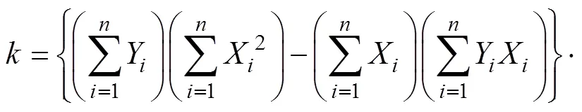
whereX=ln(V),Y=ln[−ln(1−Pv)].

Rayleigh distribution is a particular case of Weibull distribution (Carta., 2009), thus similarly, its parametercan be estimated by

For mixture distributions, the initial iteration value of the parameters of Weibull and Rayleigh can be set by Eqs. (19) and (20); as for the truncated normal from below distribution, its moment estimation is related to the first three order moments (Cohen, 1950), which can be approximately estimated by

whereas the initial iteration value of0is set as 0.5.

In meteorology, wind direction is measured using North as the starting orientation. However, in this study, the starting orientation was defined as North left 11.25 degrees; thus, the bounds of 16 directions are 11.25, 33.75, 56.25, ···, 348.75 degrees in a clockwise direction. The vector of interval wind speed frequency statistics=[1,2, ···,16] can be calculated through Eq. (22).

For the wind rose with,pd=pd/(1−). The vector of directional cumulative probability statisticsis given by Eq. (23).

To estimate parameters accurately, the wind direction distribution was fit by two steps. First, the NLSM method is used to fit the interval frequency, estimating the parameters of a mixture distribution with eight components. The initial iteration values of weight parameters are given by

The initial iteration values ofκandμare related to sandc(Carta., 2008a), which represent the mean sine and cosine values; in this study, we calculate sandcthrough Eq. (25).

Second, the components whose weight parameters are close to zero are deleted, and the cumulative probabilityis fitted by using the CDF of the mixture distribution with the residual components; in this process, the residual components’ parameters are taken as the initial iteration value.

2.6 Parameter Estimation Method of Joint Variable

For the wind rose, the collected wind data are grouped by×16 cells. Wind data whose speed and direction range fromV−1toVandθ−1toθ, respectively, are divided into the cell namedC. If the marginal distributions of wind speed and direction have been obtained, then asF() andΘ() increase monotonously, the value of joint variableinCranges from1to2according to Eq. (11). In addition, the eigenvalues1and2are only related toF(V−1),F(V) andΘ(θ−1),Θ(θ). Thus, the distance between2and1usually would not so far making the value of2−1is small. Assume an eigenvalueψrepresents the mean value offor theth scale wind happening in theth direction, andψandpjointly influence the distribution of joint variable. If this hypothesis is true, then when estimating the distribution of a joint variable, calculatingψis unnecessary because a set of simulative data that can reflect the correlation between wind speed and direction would be enough. Thus, the parameters of a joint variable can be estimated in three steps:

First,sets of wind data containing wind speed and direction are generated. For every cellC, a vector of pseudorandom numbers, of which the cumulative probability ranges fromF(V−1) toF(V), with a capacity of×pfollowing the wind speed distributionshould be generated. The same work is performed for the marginal distribution of wind direction to obtain the pseudorandom numbers vector. The simulative dataD=[θ] corresponding to cellCis defined. After all the simulative data of×16 cells have been obtained,Dis combined to.

Second,+or–is calculated for every paired data ofby utilizing the marginal distributions constructed before and Eq. (13). Afterward, the NLSM method (Madsen., 2004) is adopted to estimate the parameters1,1,2,2of the von Mises distribution1(+;1,1) and2(–;2,2) with datasets+and–, respectively;

Lastly, letω=N/,=1 and 2, in which1and2are the capacity of datasets+and–. Regarding Eq. (15) as the theoretical distribution of joint variableand taking all+and–as the simulative data, we can estimate the parameters. In the process, a numerical algorithm is applied, and1,1,1,2,2, and2are taken as the initial value of iteration.

2.7 Goodness-of-Fit Evaluation Criteria

The raw data obtained from wind rose is grouped by speed and direction. To select the optimal distribution for linear variables and validate the performance of the angular marginal distribution, this study utilizes five error metrics, including Kolmogorov-Smirnov distance (), root mean square error (), mean absolute error (), relative root mean square error (), and index of agreement ().,, andare applied to linear variables; among the four linear distributions, the one with the lowest test statistics is selected as the optimal distribution. For angular variables,,, andare used to verify if the angular distribution fits the data well. The model accuracy is divided into four levels on the basis of, which is considered excellent if<10%, good when 10%<<20%, fair when 20%<<30%, and poor when³30% (Mohammadi., 2016). As for, which varies from 0 to 1, the bigger value means the better fitting performance. These criteria can be calculated by Eq. (26).

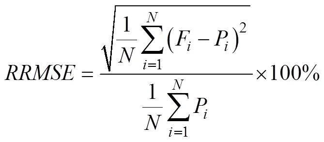
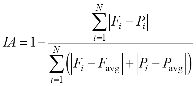
whereFdenotes theth theoretical cumulative probability;Pis the empirical cumulative probability;avgandavgrepresent the mean ofFandP, respectively;denotes the quantity of the sample.

Two kinds of coefficient of determination are listed in Eq. (27), in whichR2reflects how well the model fits the raw interval frequency, whereasR2shows the strength of the correlation about the joint cumulative probability between the model and original wind rose.

2.8 Pseudorandom Number Generation Algorithm

Compared with the simulation of the linear or angular marginal distribution, generating angular-linear paired pseu-dorandom numbers is much more difficult. The most com- mon method is based on conditional probability for multivariables (Cambou., 2015); however, for the joint probability distribution model, this method is difficult because the conditional probability function is complex. In this section, an exact algorithm generating pseudorandom numbers of paired wind speed and direction is proposed by using only the univariate distribution. The generation algorithm is shown in Fig.1. The variablesandare the mean value and concentration parameters of the finite mixture distributions of wind direction, respectively.

For a givenF()=1, Step 2 is the process of obtaining the pseudorandom number+or–, which belongs to the distribution of joint variable. The utilized method of generating the pseudorandom number of von Mises distribution is proposed by Yuan and Kalbleisch (2000). Then,by definition Eq. (13), we obtain the only and correspondingΘ().

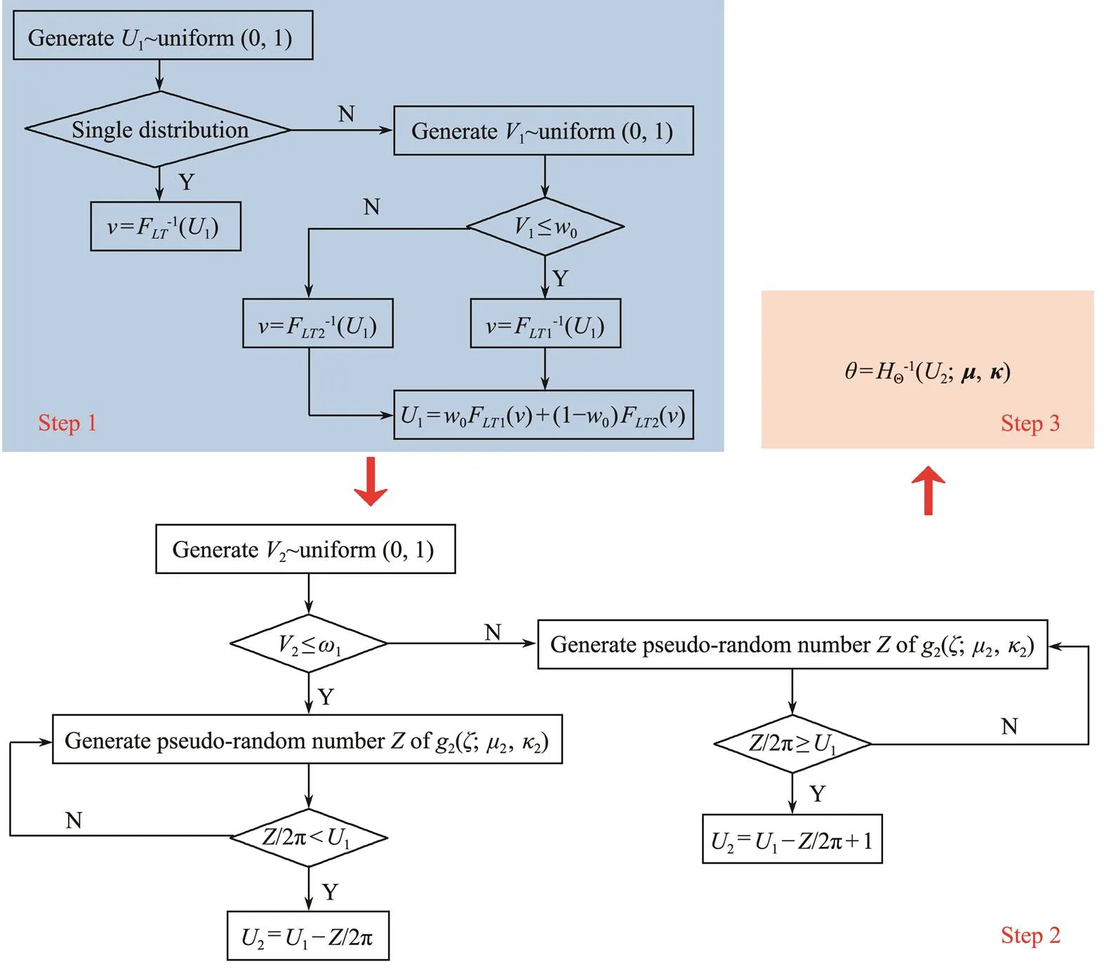
Fig.1 Generation algorithm of pseudorandom numbers.

2.9 Extreme Wind Speed Estimations

The commonly used extreme wind speed distributions, including generalized extreme value(GEV), lognormal, and Gumbel, are used to fit the selected extreme wind speed.The maximum likelihood method is applied to estimate the parameters. Cramer-von Mises statistic2, Anderson-Darling statistic2(Laio, 2004), and Akaike information criterion AIC (Akaike, 1998), are utilized to evaluate the performance of the distributions, which can be calculated as follows:

,(28b)

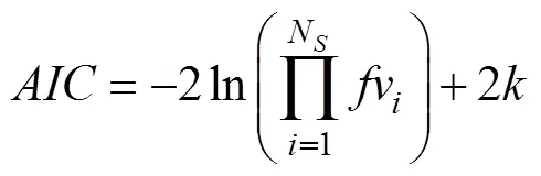
whereFvandfvrepresent theoretical cumulative probability and probability density, respectively;Nis the number of selected samples;denotes the number of parameters. The lowest value of these criteria indicates that the distribution that models the data best. To select the optimal distribution, we utilize a comprehensive metricM, which was proposed by Erdem. (2010), to evaluate the overall performance of distributions by combining the aforementioned individual statistics. The formula of the new metric can be written as follows:

whereMrepresents the original value of the statistic;MminandMmaxdenote the minimum and maximum ofM, respectively.

3 Case Study

3.1 Wind Roses Used

To validate the flexibility of the proposed model, a case study is conducted using the wind roses collected from the Changxingdao and Lüshun weather stations located in the Liaodong Gulf. The wind roses shown in Fig.2 are drawn by one year and per-three-hour mean data.

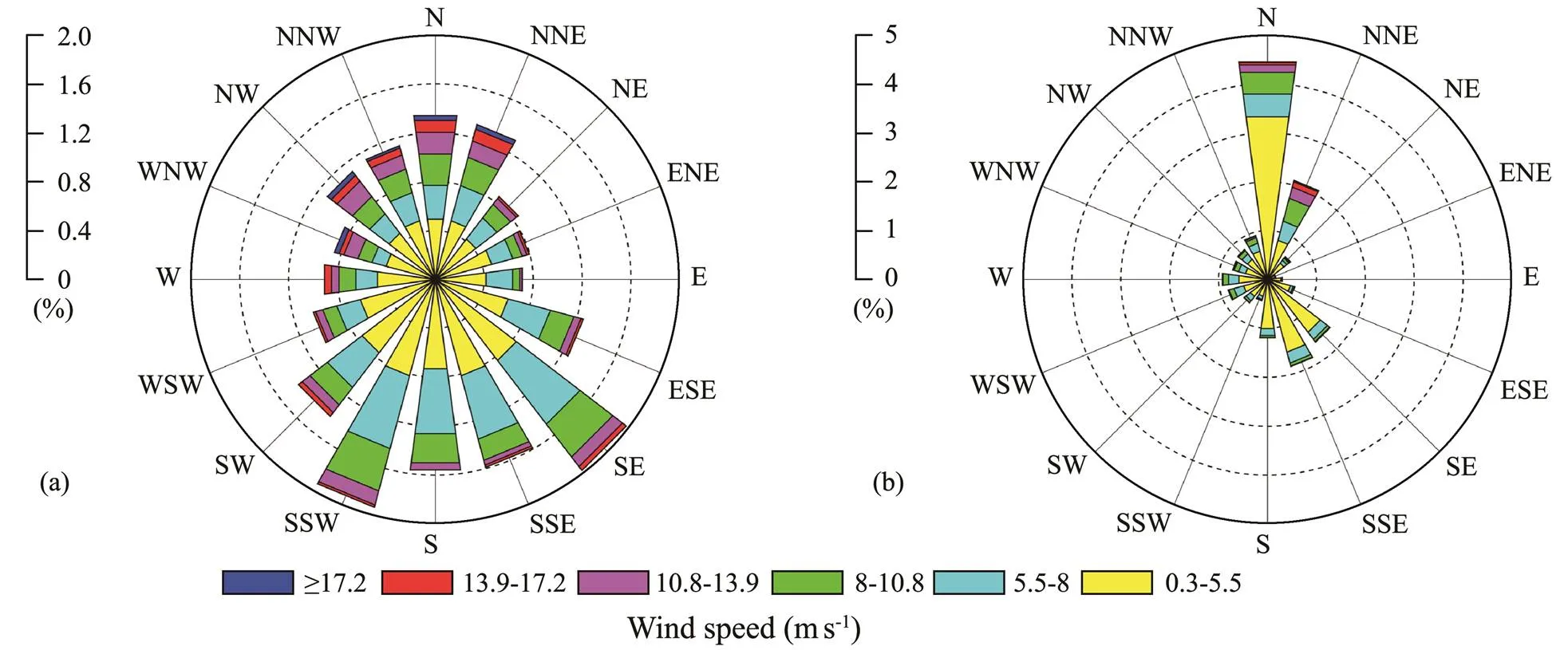
Fig.2 Wind roses of the two weather stations: (a), Changxingdao; (b), Lüshun.

3.2 Marginal Distributions of Wind Speed and Direction

To obtain the optimal wind speed distribution, LTW, LTR, MLTWR, and MLTWTN are used to fit the wind speed data.

For the Changxingdao weather station, Table 1 shows the fitting results of grouped wind speed data. Among the four alternative distributions, only the MLTWTN owns the lowest test statistics. Furthermore,is far less than the critical value of the Kolmogorov-Smirnov test statis-tics5,0.05=0.565 corresponding to the sample size of 5 and significance level of 0.05. Hence, MLTWTN is chosen to be the marginal distribution of wind speed. Fig.3(a) shows the fitting plot of grouped wind speed data; the solid red line represents the MLTWTN distribution, and the red dashed line denotes the lower-truncated truncated normal from below distribution. Moreover, the two components of the mixed distribution can be seen as two sub- models, which are also plotted by dashed lines with the same color as the parent models, representing the extreme and normal process.

Table 1 Fitting results of wind speed distributions for the Changxingdao weather station

Note:0is the weight parameter of LTW in the mixed model.

Fig.3 Fitting plots of the marginal distributions fitted for grouped wind speed data. (a), Changxingdao; (b), Lüshun.

As for Lüshun, the fitting results are shown in Table 2. Among the four alternatives, MLTWR has the lowest test statistics, and itsis much less than5,0.05=0.565. Hence, MLTWR supported by all criteria is selected as the optimal marginal distribution of wind speed. Fig.3(b) shows the graph of the mixed distribution. As shown in the figure, the LTW model has a major influence on the parent model, demonstrating that the LTW model has an advantage in modeling wind speed.

The fitting results of two weather stations show that mixture distributions outperform single distributions in modeling wind speed.

For marginal distribution of wind direction, we obtain a mixture of six von Mises (MvM6) distributions for the Changxingdao weather station, following the two-step NL- SM method. The estimated parameters are listed in Table 3. As for Lüshun, a mixture of four von Mises (MvM4) distributions is obtained, and the corresponding parameters are shown in Table 4. The values of statistics,,of the two weather stations in the test process are presented in Table 5.is far less than16,0.05=0.327; moreover,<10%, andis close to 1, proving that the model accuracy is excellent. Thus, the proposed method achieves great fitness to the grouped wind direction data. Figs.4(a) and (b) are the fitting plots of grouped wind direction data.

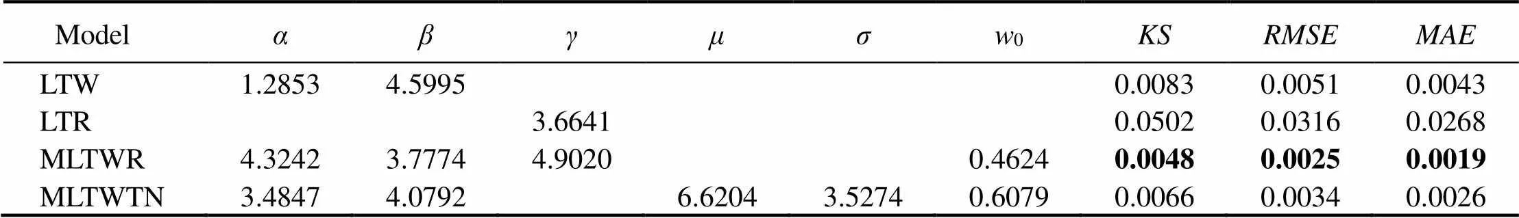
Table 2 Fitting results of wind speed distributions for the Lüshun weather station

Note:0is the weight parameter of LTW in the mixed model.

Table 3 Parameters of wind direction distribution for the Changxingdao weather station

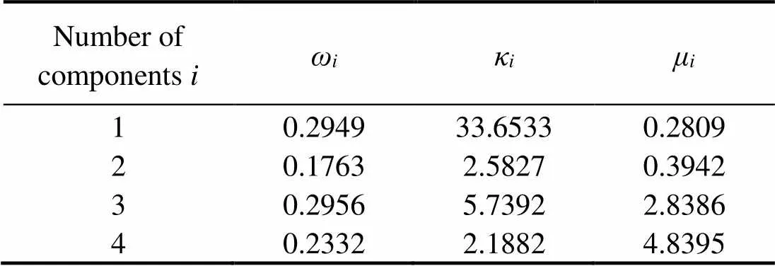
Table 4 Parameters of wind direction distribution for the Lüshun weather station

Table 5 Performance evaluation of wind direction distributions

3.3 Distribution of the Joint Variable

In Subsection 2.6, a method is proposed to estimate the parameters of the distribution of joint variables without researching the influence of the capacity of the simulative data. Thus, after the marginal distributions have been obtained, 10 sets of simulative data are generated for each case with the capacity of 1000, 2000, 3000, 4000, 5000, 6000, 7000, 9000, 12000, and 15000. On the basis of every estimated distribution of a joint variable, models marked as M1000, M2000, ···, M15000for the joint distribution of wind speed and direction are obtained. The two kinds of coefficient of determination are applied to assess the fit- ness of these models.

Fig.4 Fitting plots of the marginal distributions fitted for grouped wind direction data. (a), Changxingdao; (b), Lüshun.

Table 6 shows the results ofR2andR2for two cases. The capacity of the simulative data does not influence the strength of correlation in both cases, indicating that increasing the capacity does not help improve the fitting performance. Nevertheless, the results of the two kinds of coefficient are perfect for every model, meaning the parameters of joint variable distribution can be well estimated by the proposed method.

Lastly, for the Changxingdao weather station, M6000is chosen as the optimal model, withR2=0.9991 andR2=0.9377, which are good enough to prove that the model is related to the wind rose tightly. As for the models of Lü- shun, the evaluation statistics of M7000,,R2=0.9983 andR2=0.9527, are over 95%, which means that the model has a strong correlation with the wind rose. The parameters of the joint variable distribution for the two models are shown in Table 7. Fig.5 presents the graph about the Changxingdao weather station; Fig.5(a) represents the theoretical joint cumulative probabilityagainst the em- pirical value, whereas Fig.5(b) is about interval frequency,against. The same graphs are shown in Fig.6 but for the case of Lüshun.

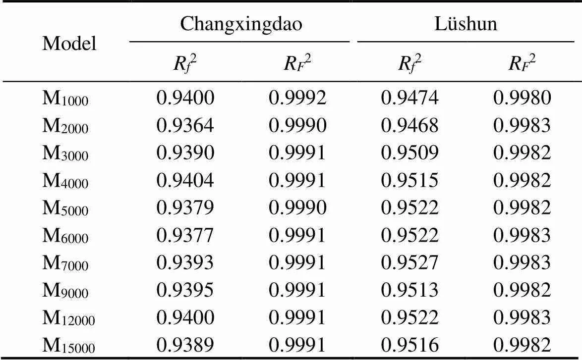
Table 6 Performance evaluation of joint variable distributions

Table 7 Parameters of joint variable distributions

Fig.5 Goodness-of-fit plots for the joint variable distribution of the Changxingdao weather station.

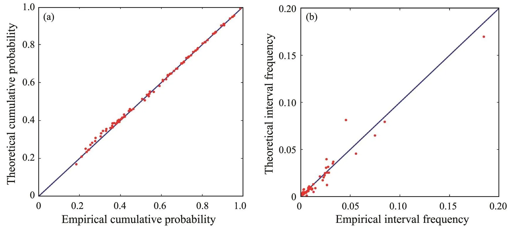
Fig.6 Goodness-of-fit plots for the joint variable distribution of the Lüshun weather station.

3.4 Graph of the Joint Probability of Wind Speed and Direction

Using the built models, we define the following in the cylindrical coordinate system (,,):as wind speed,as the direction of the wind, andas the cumulative frequency of wind whose speed is underand happening in the interval with a wind direction ranging from (−11.25) degrees to (+11.25) degrees; the value ofandare taken in their domain continuously. In the plane graph (,), let the color change with the value of. By using the constructed models to calculate this three-dimensionalarray, a new kind of graph, which can reflect the joint probability distribution of wind speed and direction continuously, is plotted (Fig.7).

Compared with the traditional wind roses shown in Fig.2,the new graphs of the joint probability distribution are continuous on speed and direction, of which the joint distributioncharacteristicscanbedescribedmoreaccurately.More-over,theyaremuchsimilartotheoriginalwindroses,prov- ing that the built model can model the joint probability dis- tribution of wind speed and direction well.

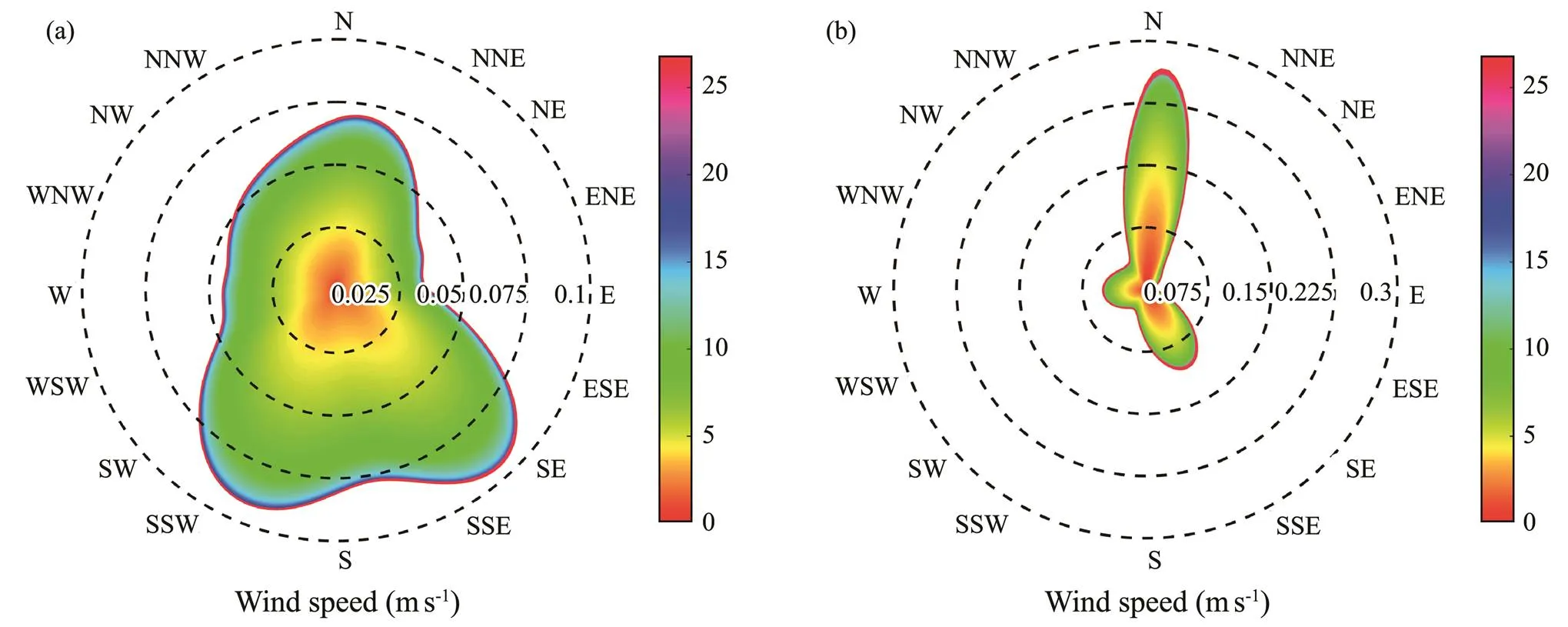
Fig.7 Joint probability distribution plots of the two weather stations. (a), Changxingdao; (b), Lüshun.

3.5 Evaluation of Wind Energy Potential

In the field of wind energy exploitation, some research must be conducted on certain wind characteristics, among which valid wind power density (), annual energy output (), and capacity factor () are key factors. They are crucial for the evaluation of wind resources and essential for the selection and performance evaluation of wind turbines. Given that the hub height (H), cut-in speed (in), and cut-out speed (out), which are related to theabove-mentioned wind characteristics, vary from different turbine models, this study selects the four latest turbine models from http://en.wind-turbine-models.com/ for subsequent research; their properties are given in Table 8. The formulation expressed in Eq. (30) is used for calculation due to the lack of power curves (Wang., 2016).

wherePdenotes the rated power of a specific wind turbine model, of whichP() represents the power at, andvrepresents the rated speed. Moreover,() is the coefficient of the output power of wind turbines when the wind speed is betweeninandout. In recent years, scholars proposed several function models (Wang., 2016) to approximate(), which are listed and plotted in Fig.8. Here, the average of the functions of() is adopted to remove the effects caused by the differences of functions.

Table 8 Properties of the wind turbine models

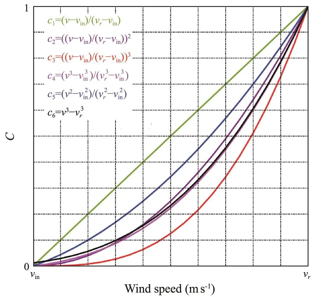
Fig.8 Function models and their plots of c(v).

3.5.1 Valid wind power density

Wind turbines generate wind power when the wind speed is valid, that is, betweeninandout; thus, conducting some research on the distribution ofin the early-stage preparation is beneficial. In addition, the influence of wind speed onis conspicuous owing to its cubic relationship; a more precise result can be obtained if the joint probability distribution, instead of the mean wind speed not considering direction, is used in the calculation. In accordance with the formula of wind power density calculation (Liu., 2019), the equation ofcombined with joint probability distribution is given by

whereis the air density, assuming to be 1.225kgm−3;vdenotes wind speed at theH.

However, the joint distribution obtained before is suita- ble for the wind speed and direction at the height of 10m, which is the height of an anemometer. Wind speed is trans-formed by the following equation (Adaramola., 2011):

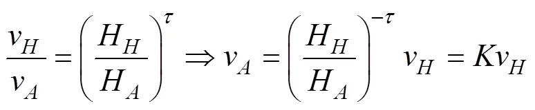
whereis the surface roughness (in most cases, it is set as 0.143 (Adaramola., 2011)), andvrepresents wind speed at the height ofthe anemometer. Then, Eq. (31) can be rewritten as

The results of calculatedare presented in Table 9, which reveals that theincreases with the increase in HH and increases to approximately 300Wm−2when the HH changes from 80m to 135m. Compared with the results of the Changxingdao weather station, theof Lüshun does not vary much when theHchanges the same because the probability of valid wind speed is low even if the height changes. Fig.9 shows the graphs of the distribution offor the two cases at differentHof 80, 120, 135, and 100m, corresponding to the selected wind turbine models. Fig.9(a) reveals that valid wind power is mainly concentrated on the SSW-SW, SSE, and NNE directions at Changxingdao. As for the case of Lüshun, Fig.9(b) shows that its valid wind power exists in the N-NNE directions. With the increase inH, the existing highest wind speed becomes less thanout, making a waste of wind turbines.

Table 9 VWPD (Wm−2) of the two weather stations at different hub heights

3.5.2 Annual energy output

As another important index in evaluating wind energy potential,reflects the amount of electrical energy that a specific wind turbine can generate over a year. By combining the joint probability distribution, thecan be defined as

where T=365×24=8760 denotes the number of hours over one year.

Valid wind speedvÎ[in,out] and wind directionÎ[0, 2π) are discrete to arithmetic progression (v,=1, 2, ···,) and (,=1, 2, ···,), respectively. Thecan be approximately calculated with the formula below, thereby saving time and computer resources when performing numerical computation.

∆vand ∆θdenote the tolerance of wind speed and direction, respectively. From Feng and Shen (2015), the arithmetic solution ofbecomes bigger than the actual value and fluctuates significantly when ∆θexceeds 1 degree and changes. By contrast, it is not sensitive to the change of ∆v. Thus, to estimateaccurately, we set ∆v=1ms−1and ∆θ=1˚.

Theof four different turbine models at the two stations is shown in Table 10, which reveals that the high- est value ofat the Changxingdao weather station is 32.81GWh, whereas the lowest value is 11.07GWh; the corresponding values are 15.61 and 5.48GWh for Lüshun. Therefore, Changxingdao is more promising than Lüshun for wind energy exploitation. At a fixed site, the trend is thatincreases with rated power growing, except for M.3, which is caused by its highest rated speed. Moreover, from the directionalof the two weather stations shown in Fig.10, a big difference exists among the 16 directions in. With the rated power growing, the difference becomes bigger, implying the significance of considering direction when evaluating wind resources.

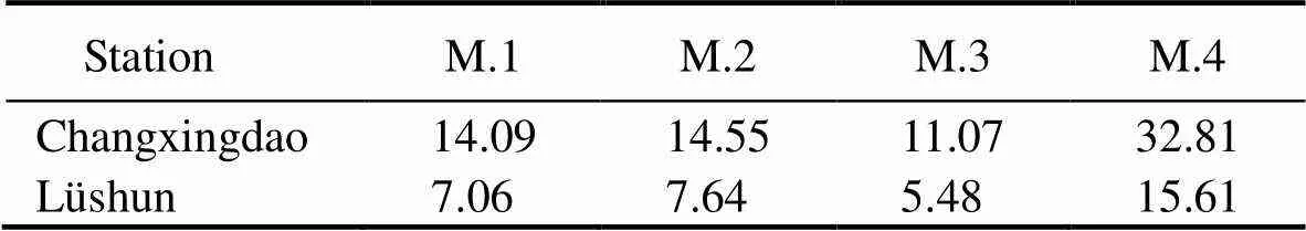
Table 10 AEO (GWh) of different wind turbine models at two weather stations

3.5.3 Capacity factor

For wind turbines,is an important factor reflecting the ability to convert wind power resources into electricity (Wang., 2016). Moreover, it is a crucial reference index when choosing wind turbines and can be calculated by

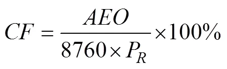
Table 11 lists the CF of different wind turbine models at the two weather stations. Overall, the CF of the Chang- xingdao weather station is higher than that of Lüshun due to having a better wind condition. For either of the two stations, M.4 owns the highest CF for the lower rated speed and higher rated power, whereas the CF of M.3 is the lowest due to its too high rated speed, making the working hours at its rated power small.

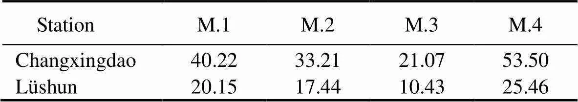
Table 11 CF (%) of different wind turbine models at two weather stations

3.6 Directional Extreme Wind Speed Under Different Return Periods

In practical engineering, extremes are important factors that any design cannot ignore. In Subsection 2.8, an algorithm is proposed to generate pseudorandom numbers of the joint distribution model. After the models for the two stations have been obtained, the model is used to generate pseudorandom wind data to predict the directional extreme wind. Simulation is performed 100 times for each case. During every simulation, 2920 pseudorandom wind data are generated, the capacity of which is equal to the data that the wind roses are drawn by, and the annual directional extremes are picked out. Fig.11 shows the boxplots of the simulated annual directional extremes for the Changxingdao and Lüshun weather stations. The boxplots of the two weather stations reveal that for most directions, the observed extremes fall in the simulated intervals of the valid maximum and minimum. Among the observed data fall out of its most extreme interval, most of them, except NNE, NE, and NNW of the Lüshun weather station, are close to their valid maximum, minimum, or outlier, proving that the simulation can predict the very extreme wind regime well. In accordance with these, the feasibility of the simulation of annual directional extremes is validated.

The simulated wind data are then used to calculate the extreme wind speed under different return periods using the directional annual extreme wind speed and the extreme wind speed ignoring direction separately.

Table 12 shows the fitting results, which reveal that for different directions, the optimal curve is not constant. More-over, the Gumbel distribution provides the best fit for 37.5% (12 of 32) directions of the two stations and is also selected as the optimal model for annual extreme wind speed mark- ed as ‘ALL’, proving that the accuracy of the Gumbel model is the best among the selected distributions in modeling extreme wind speed data, followed by the lognormal model; GEV is considered to have the worst distribution as it provides least favorable fits to the directional extreme wind speed data of the selected stations.

Figs.12 and 13 show the optimal distribution curves of 16 directions for the Changxingdao and Lüshun weather stations, respectively. The fitting curves of wind speed ignoring direction can be obtained from Fig.14.

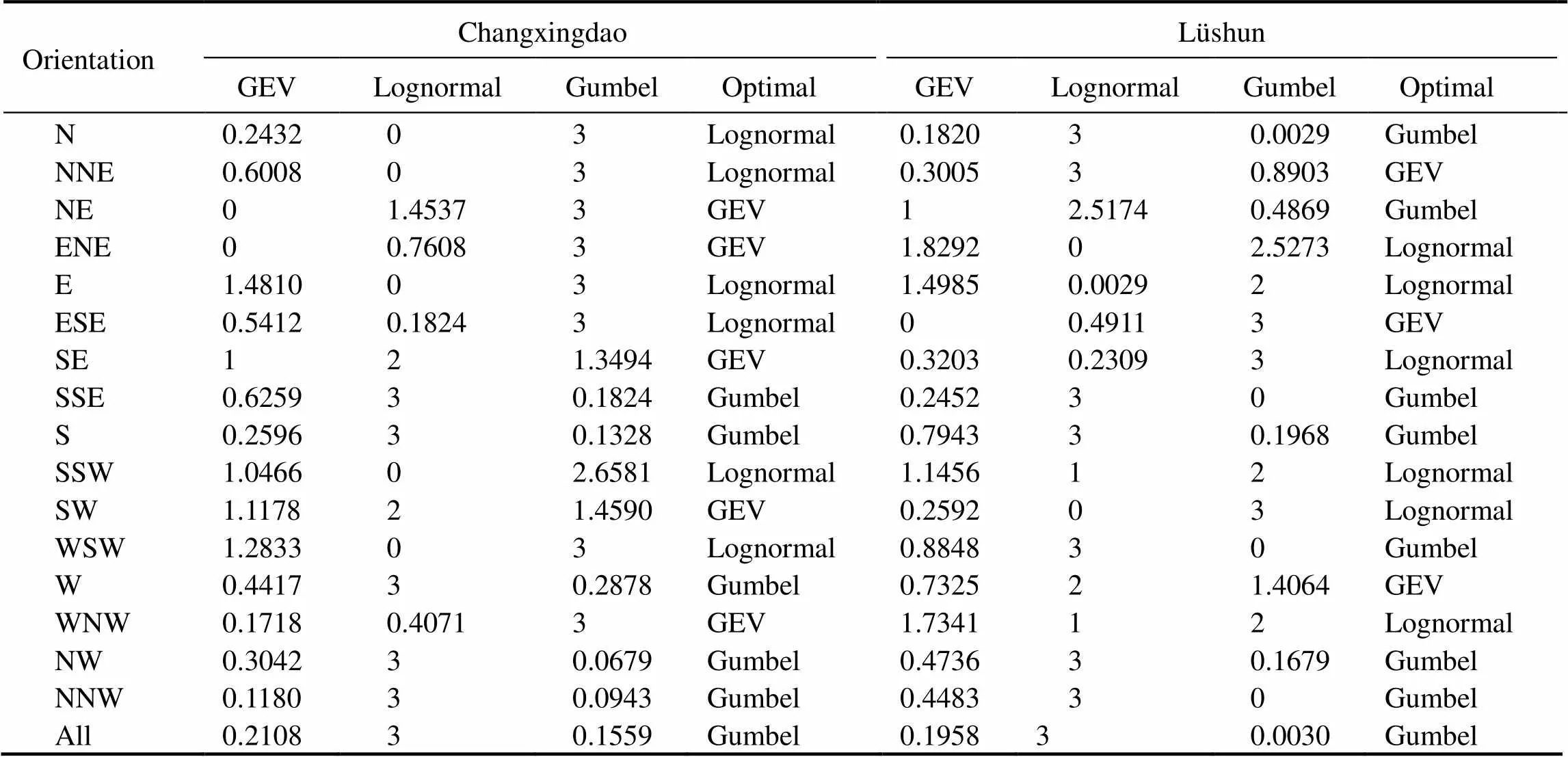
Table 12 Fitting results of annual extreme wind speed for the two weather stations

Fig.11 Simulation of annual directional extreme wind speed. (a), Changxingdao; (b), Lüshun.

Fig.12 Fitting curves of the annual directional extreme wind speed of the Changxingdao weather station.

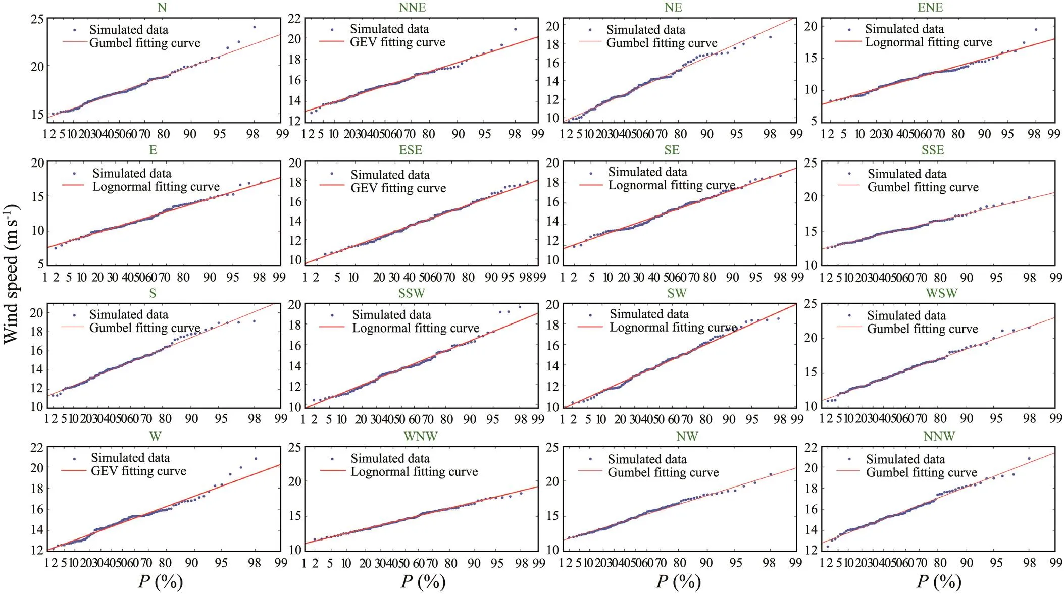
Fig.13 Fitting curves of the annual directional extreme wind speed of the Lüshun weather station.

Fig.14 Fitting curves of extreme wind speed ignoring the direction of the two weather stations. (a), Changxingdao; (b), Lüshun.

Lastly, both the extreme wind speed estimated respectively for 16 directions and that estimated ignoring the influence of direction at selected weather stations under return periods of 10, 20, 50, and 100 years are plotted in Fig.15, in which the unit of wind speed is ms−1.

The prevailing regions of a wind field are likely occurring dangerous extreme wind; however, as shown in Fig. 15, some directions with low wind frequency have extreme wind speeds that are strong, especially when the return period increases. This phenomenon may indicate potentially dangerous wind directions that should be treated care- fully in practice. Moreover, the extreme wind speed estimated by directional speed data is lower than that estimated by data ignoring direction, especially for the Changxingdao weather station with several prevailing wind directions. This finding suggests that the cost can be reduced if the design wind speed for wind turbines is determined by that estimated using directional wind speed data. Further discussion is needed for the case of Lüshun, where the estimated annual directional extreme wind speeds under the return period of 100 years of its prevailing regions are a little less than the observed extreme wind speed. This result may be attributed to the fact that the length of the wind data used to make the wind rose is not long enough to represent the overall meteorological characteristics of the wind field.

Fig.15 Estimated extreme wind speed under different return periods for Changxingdao (upper panel) and Lüshun (lower panel).

4 Conclusions

With the application of the proposed model in analyzing the wind roses of two weather stations in the Liaodong Gulf, the following conclusions are drawn:

1) The proposed model to build the joint probability distribution of wind speed and direction gives a more accurate distribution of the wind condition compared with windrose.Furthermore,itcangeneratepseudorandomnumbers of wind speed and paired direction with the algorithm presented.

2) Lower-truncated distribution is fit for grouped data from wind roses; compared with single distributions of wind speed, the mixed distribution shows more flexibility and precision.

3) The proposed two-step NLSM method can accurately fit the distribution of wind direction in zones with several prevailing wind directions by using grouped data. In addition, the novel simulation method to estimate the parameters of the joint variable distribution can provide enough precision without requiring the generation of large simulative data.

4) The constructed model can be used for several tasks, including the evaluation process of the available wind energy resources considering the influence of direction at a potential site.

5) The constructed model can approximately predict the annual directional extreme wind speed under different return periods combining with Monte Carlo simulation. The predicted extreme wind speed is less than that estimated by data ignoring direction under the condition that the wind rose can represent the meteorological characters of the wind field well.

Acknowledgements

The study was supported by the National Key Research and Development Program of China (No. 2016YFC0303401), the National Natural Science Foundation of China (No. 51779236), and the National Natural Science Foundation of China–Shandong Joint Fund (No. U1706226).

Adaramola, M. S., Paul, S. S., and Oyedepo, S. O., 2011. Assessment of electricity generation and energy cost of wind energy conversion systems in north-central Nigeria., 52 (12): 3363-3368.

Akaike, H., 1998. Information theory and an extension of the maximum likelihood principle. In:. Parzen, E.,, eds., Springer Series in Statistics, Springer, New York, 199-213.

Akdağ, S. A., Bagiorgas, H. S., and Mihalakakou, G., 2010. Use of two-component Weibull mixtures in the analysis of wind speed in the eastern Mediterranean., 87: 2566-2573.

Allouhi, A., Zamzoum, O., Islam, M. R., Saidur, R., Kousksou, T., Jamil, A.,, 2017. Evaluation of wind energy potential in Morocco’s coastal regions., 72: 311-324.

Alsaad, M. A., 2013. Wind energy potential in selected areas in Jordan., 65: 704-708.

Cambou, M., Hofert, M., and Lemieux, C., 2015. Quasi-random numbers for copula models., 27: 1-23.

Carta, J. A., and Ramírez, P., 2007a. Analysis of two-component mixture Weibull statistics for estimation of wind speed distributions., 32: 518-531.

Carta, J. A., and Ramírez, P., 2007b. Use of finite mixture distribution models in the analysis of wind energy in the Canarian Archipelago., 48: 281-291.

Carta, J. A., Bueno, C., and Ramírez, P., 2008a. Statistical modelling of directional wind speeds using mixtures of von Mises distributions: Case study., 49: 897-907.

Carta, J. A., Ramírez, P., and Bueno, C., 2008b. A joint probability density function of wind speed and direction for wind energy analysis., 49: 1309-1320.

Carta, J. A., Ramírez, P., and Velázquez, S., 2009. A review of wind speed probability distributions used in wind energy analysis: Case studies in the Canary Islands., 13: 933-955.

Cohen, A. C., 1950. On estimation the mean and variance of singly truncated normal frequency distributions from the first three samples moments., 3: 37-44.

Cook, N. J., 2019. The OEN mixture model for the joint distribution of wind speed and direction: A globally applicable model with physical justification., 191: 141-158.

Erdem, E., and Shi, J., 2011. Comparison of bivariate distribution construction approaches for analyzing wind speed and direction data., 14: 27-41.

Erdem, E., Li, G., and Shi, J., 2010. Comprehensive evaluation of wind speed distribution models: A case study for North Dakota sites., 51 (7): 1449-1458.

Feng, J., and Shen, W. Z., 2015. Modelling wind for wind farm layout optimization using joint distribution of wind speed and wind direction., 8: 3075-3092.

Han, Q. K., Hao, Z. L., Hu, T., and Chu, F. L., 2018. Non-parametric models for joint probabilistic distributions of wind speed and direction data., 126: 1032-1042.

Han, Q. K., Ma, S., Wang, T. Y., and Chu, F. L., 2019. Kernel density estimation model for wind speed probability distribution with applicability to wind energy assessment in China., 115: 109387.

Huang, S., and Wan, H., 2012. Determination of suitability between wind turbine generators and sites including power density and capacity factor considerations., 3 (3): 390-397.

Jaramillo, O. A., and Borja, M. A., 2004. BimodalWeibull wind speed distributions: An analysis of wind energy potential in La Venta, Mexico., 28 (2): 225-234.

Johnson, R. A., and Wehrly, T. E., 1978. Some angular-linear distributions and related regression models., 73 (363): 602-606.

Justus, C. G., Hargraves, W. R., Mikhail, A., and Graber, D., 1978. Methods for estimating wind speed frequency distributions., 17 (3): 350-353.

Kantar, Y. M., and Usta, I., 2015. Analysis of the upper-truncated Weibull distribution for wind speed., 96: 81-88.

Keyhani, A., Ghasemi-Varnamkhasti, M., Khanali, M., and Abb- aszadeh, R., 2010. An assessment of wind energy potential as a power generation source in the capital of Iran, Tehran., 35: 188-201.

Koeppl, G. W., 1982.. 2nd edition. Van Nostrand Reinhold, New York, 67-89.

Laio, F., 2004. Carmer-von Mises and Anderson-Darling goodness of fit tests for extreme value distributions with unknown parameters., 40: W09308.

Li, H. N., Zheng, X. W., and Li, C., 2019. Copula-based joint distribution analysis of wind speed and direction., 145 (5): 04019024.

Li, Z. Q., Chen, S. J., Ma, H., and Feng, T., 2013. Design defect of wind turbine operating in typhoon activity zone., 27: 165-172.

Liu, F., Sun, F. B., Liu, W. B., Wang, T. T., Wang, H., Wang, X. M.,, 2019. On wind speed pattern and energy potential in China., 236: 867-876.

Madsen, K., Nielsen, H. B., and Tingleff, O., 2004.. Technical University of Denmark, Denmark, 1-49.

Masseran, N., Razali, A. M., and Ibrahim, K., 2012. An analysis of wind power density derived from several wind speed density functions: The regional assessment on wind power in Malaysia., 16: 6476-6487.

Masseran, N., Razali, A. M., Ibrahim, K., and Latif, M. T., 2013. Fitting a mixture of von Mises distributions in order to model data on wind direction in Peninsular Malaysia., 72: 94-102.

Mazzeo, D., Oliveti, G., and Labonia, E., 2018. Estimation of wind speed probability density function using a mixture of two truncated normal distributions., 115: 1260-1280.

McWilliams, B., and Sprevak, D., 1980. The estimation of the parameters of the distribution of wind speed and direction., 4: 227-238.

McWilliams, B., Newmann, M. M., and Sprevak, D., 1979. The probability distribution of wind velocity and direction., 3: 269-273.

Mirhosseini, M., Sharifi, F., and Sedaghat, A., 2011. Assessing the wind energy potential locations in province of Semnan in Iran., 15: 449-459.

Mohammadi, K., Alavi, O., Mostafaeipour, A., Goudarzi, N., and Jalilvan, M., 2016. Assessing different parameters estimation methods of Weibull distribution to compute wind power density., 108: 322-335.

Ovgor, B., Lee, S., and Lee, S., 2012. A method of micrositing of wind turbine on building roof-top by using joint distribution of wind speed and direction, and computational fluid dynamics., 26 (12): 3981-3988.

Pishgar-Komleh, S. H., Keyhani, A., and Sefeedpari, P., 2015.

Wind speed and power density analysis based on Weibull and Rayleigh distributions (a case study: Firouzkooh county of Iran)., 42: 313-322.

Qin, X., Zhang, J. S., and Yan, X. D., 2010. A new circular distribution and its application to wind data., 2 (3): 12.

Schindler, D., and Jung, C., 2018. Copula-based estimation of directional wind energy yield: A case study from Germany., 169: 359-370.

Stephen, B., Galloway, S., McMillan, D., Anderson, L., and Ault, G., 2013. Statistical profiling of site wind resource speed and directional characteristics., 7 (6): 583-592.

Tiang, T. L., and Ishak, D., 2012. Technical review of wind energy potential as small-scale power generation sources in Penang Island Malaysia., 16: 3034-3042.

Vanem, E., Hafver, A., and Nalvarte, G., 2020. Environmental contours for circular-linear variables based on the direct sampling method., 23: 563-574.

Wang, J. Z., Hu, J. M., and Ma, K. L., 2016. Wind speed probability distribution estimation and wind energy assessment., 60: 881-899.

Wang, J. Z., Qin, S. S., Jin, S. Q., and Wu, J., 2015. Estimation methods review and analysis of offshore extreme wind speeds and wind energy resources., 42: 26-42.

Weber, R., 1991. Estimator for the standard deviation of wind direction based on moments of the Cartesian components., 30 (9): 1341-1353.

Weber, R., 1997. Estimators for the standard deviation of horizontal wind direction., 36: 1407-1415.

Ye, X. W., Xi, P. S., and Nagode, M., 2019. Extension of REB- MIX algorithm to von Mises parametric family for modeling joint distribution of wind speed and direction., 183: 1134-1145.

Yuan, L., and Kalbfleisch, J. D., 2000. On the Bessel distribution and related problems., 52 (3): 438-447.

Zhang, J., Chowdhury, S., Messac, A., and Castillo, L., 2013. A multivariate and multimodal wind distribution model., 51: 436-477.

November 30, 2020;

March 15, 2021;

April 19, 2021

© Ocean University of China, Science Press and Springer-Verlag GmbH Germany 2022

. Tel: 0086-532-66781125

E-mail: dongsh@ouc.edu.cn

(Edited by Xie Jun)