Efficient Computational Approach for Predicting the 3D Acoustic Radiation of the Elastic Structure in Pekeris Waveguides

QIAN Zhiwen, HE Yuanan, SHANG Dejiang, ZHAO Haihan, and ZHAI Jingsheng, *

Efficient Computational Approach for Predicting the 3D Acoustic Radiation of the Elastic Structure in Pekeris Waveguides

QIAN Zhiwen1), HE Yuanan2), SHANG Dejiang3), ZHAO Haihan1), and ZHAI Jingsheng1), *

1) School of Marine Science and Technology, Tianjin University, Tianjin 300072, China 2) Systems Engineering Research Institute, Beijing 100036, China 3) College of Underwater Acoustics Engineering, Harbin Engineering University, Harbin150001, China

Ocean boundaries present a significant effect on the vibroacoustic characteristics and sound propagation of an elastic structure in practice. In this study, an efficient finite element/wave superposition method (FE/WSM) for predicting the three-dimen- sional acoustic radiation from an arbitrary-shaped radiator in Pekeris waveguides with a lossy seabed is proposed. The method is based on the FE method (FEM), WSM, and sound propagation models. First, a near-field vibroacoustic model is established by the FEM to obtain vibration information on a radiator surface. Then, the WSM based on the Helmholtz boundary integral is used to pre- dict the far-field acoustic radiation and propagation. Furthermore, the rigorous image source method and complex normal mode are employed to obtain the near- and far-field Green’s function (GF), respectively. The former, which is based on the spherical wave decomposition, is adopted to accurately solve the near-field source strength, and the far-field acoustic radiation is calculated by the latter and perturbation theory. The simulations of both models are compared to theoretical wavenumber integration solutions. Finally, numerical experiments on elastic spherical and cylindrical shells in Pekeris waveguides are presented to validate the accuracy and efficiency of the proposed method. The results show that the FE/WSM is adaptable to complex radiators and ocean-acoustic envi- ronments, and are easy to implement and computationally efficient in calculating the structural vibration, acoustic radiation, and sound propagation of arbitrarily shaped radiators in practical ocean environments.

elastic structure; acoustic radiation; Pekeris waveguide; wave superposition method; Green’s function; image source method; spherical wave decomposition

1 Introduction

During the past several decades, computational meth- ods for the acoustic and vibration characteristics of elastic structures (, plates, spherical shells, and cylindrical shells) have gained considerable attention from many scholars. One of the difficulties in computational mechan- ics is the analytical modeling of coupling effects between the elastic structure and surrounding fluids,, fluid-solid interaction (FSI), which are considered in basic theories (Junger and Feit, 1986; Ma, 2015). Furthermore, the expression of the sound field radiated from an elastic structure under force (sound) excitation was developed by combining the Flügge shell theory (Pang, 2018) with the acoustic wave equation (Klaseboer, 2017), which has laid a remarkable foundation for the subsequent work on the vibroacoustic prediction of elastic structures in a complex fluid environment.

Extending from the continental shelf to the deep ocean, the extensive transition area is shallow water with a depth of fewer than 200m (Paul, 2013), and many elastic struc-tures, such as underwater vehicles, pipelines, and offshore platforms, have been deployed in this area, driving peo- ple’s awareness of the environment protection, marine sci- entific research, and military investigation. To effectively investigate research scopes, such as the near-field sound measurement, acoustic cloak design, and target identifica- tion, the acoustic radiation mechanisms of elastic struc- tures in shallow water need to be understood. Different from previous computational schemes in infinite fluids, the FSI vibration and acoustic radiation in shallow water will be significantly affected by the reflected sound of up- per and lower boundaries. First, the reflected sound field act as a counteracting excitation on the structure surface. Thus, the FSI system can be considered a sound-structure interaction (SSI) problem (Zhao and Wu, 2005). Second, the reflected sound field mixed with the direct sound field can propagate over long distances (Pan, 2014). Thus, it is difficult to perform a comprehensive model to solve the Helmholtz equation subjected to multi-boundary con- ditions and complex structural vibrations. Furthermore, the model needs to meet the highly demanding requirements that can calculate the characteristics of the near-field SSI problem and the sound field affected by the boundaries, and it also needs to describe the far-field sound propaga- tion in shallow water.

Studies on sound propagation in shallow water have generally focused on a monopole source. Many scholars have explored various sound propagation models (Jensen, 2011), such as ray theory (Liu and Li, 2019), nor- mal mode (NM) (Yang, 2016), wavenumber inte- gration (WI) method (Cockrell and Schmidt, 2010), para- bolic equation method (Xu, 2017), and some hybrid methods (Collis, 2016; Ballard, 2019). As a direct analog of the remarkable achievements in these propaga- tion models, the acoustic radiation characteristics of elas- tic structures in the far field have been investigated. How- ever, these analogy strategies do not contain geometric characteristics and the near-field SSI vibration of the elas- tic structures. Moreover, far-field acoustic calculation me- thods do not have sufficient accuracy and reliability.

Early computational methods that describe huge radia- tors as the sound source have been developed by research- ers. Bai(2014) developed a model based on the thin-shell vibration equation and traditional image source me- thod(ISM), and investigated the submerged depth on the sound field of a cylindrical shell in ideal shallow water. Furthermore, Wang(2017) presented a method based on the Flügge shell theory, wave equation, and ISM to study the influence of boundaries on low-frequency SSI vibrations. However, generally, the ISM loses its accuracy in far-field acoustic problems but is best handled by NM solutions. Based on this information, Oğuz (1996) com- bined the ISM with the NM to predict the acoustic radia- tion in shallow water. However, the premise of using the ISM is knowing the identified sound expression of a physical radiator. Therefore, these combined ISM meth- ods, in general, can only calculate the two-dimensional (2D) sound field of typical structures in ideal shallow water, and it is impractical to calculate the acoustic radiation of arbitrary elastic structures in other complex oceans. Thus, an effective hybrid approach, coupling the FEM and BEM (FE/BEM), is presented to solve the SSI problem in shal- low water with variable sound speed (Jiang, 2018). By using boundary integrals, Zou(2013) and Jiang(2020) employed the three-dimensional (3D) sonoelastic- ity theory for ships in shallow water. Benchmark examples for the integrated calculation of elastic bodies were also pro- vided. However, this approach has two disadvantages: first, numerical singular integrals will occur when the distance between the simple source and surface point becomes zero (Miller, 1991), and second, a uniqueness problem associ- ated with the resonances of the interior fluid is overcome by resourceful mathematics (Zou, 2018). These dis- advantages complicate the numerical algorithm and in- crease the coding effort in the exterior acoustic calculation. To circumvent these limitations, Koopmann(1989) introduced an easy-to-implement and computationally effi- cient method called the wave superposition method (WSM), which is suitable for calculating acoustic fields of arbi- trarily shaped radiators in complex fluid environments by adjusting the Green’s function (GF). WSM is successfully applied to acoustic radiation (Fahnline and Koopmann, 1991), scattering (Irena and Henrik, 2006), reconstruction (Ping, 2017), and the sound field in motion (Zhang, 2008), illustrating its high adaptability and efficiency in predicting the acoustic radiation in the complex fluid. Hence, Shang(2018) used the WSM to compute the structural acoustic radiation in the ideal shallow water, but the calculation accuracy needed to be improved because the GF obtained by the NM loses its accuracy for near-field problems. Moreover, the fluid is too idealistic for practi- cal ocean-acoustic environments. Thus, Zou(2020) presented a mixed method based on the analytical method, WSM, and combined GFs, where the symmetrical vibro- acoustic problems of a spherical double shell immersed in the ocean were predicted accurately. However, the ana- lytical solution is hardly adapted in asymmetric structures with arbitrary shapes, and the traditional ISM is generally designed for high-frequency and low-velocity seabed envi- ronments. Thus, to avoid the shortcomings of the methods mentioned above, it is necessary to develop a new compu- tational strategy that can be adapted to complex radiators and ocean environments and can effectively simplify the implementation complexity and improve computational efficiency.

The remarkable achievements have benefited from re- search on vibration and noise reduction technology (Zhang, 2018; Zhong, 2019), allowing high-frequency sound waves to be absorbed by special artificial materials and barring them from traveling to long distances in the ocean. Therefore, the sound field research in shallow wa- ter generally focuses on low-frequency sound propagation. In this frequency band, the FEM needs less meshing cal- culation, and the WSM requires few simple sources. There- fore, considering the advantages of the two methods and their adaptability to complex radiators and ocean environ- ments, we attempted to conduct a new computational FE/ WSM for the low-frequency acoustic radiation of arbi- trary elastic structures in a more practical ocean environ- ment. This FE/WSM is modeled by the widely used Pekeris waveguides with a lossy seabed rather than an ideal envi- ronment. This theoretical model consists of a near-field FEM for discretizing structures and a far-field WSM for calculating the sound field. Particularly, it comprises three parts: 1) Near-field FEM solution. A 3D acoustic radia- tion model is established by the multi-physics coupling FEM, and the vibration velocity on the structure surface is obtained. 2) Near-to-far field propagation model. The GF of the sound field propagation in Pekeris waveguides is solved by the rigorous ISM and NM to accurately solve the near- and far-field problems, respectively. 3) WSM calculation. An array of equivalent simple sources are op- timally configured inside the radiator, and the source strengths are solved by combining the vibration velocity with the near-field GF. Then, the sound field generated by each simple source at a receiver is summed by the far-field GF, which can be equivalent to the sound field radi- ated from the physical radiator. Finally, the results of the rigorous ISM and NM models are compared to the theo- retical solutions predicted by WI. The numerical experi- ments are modeled by COMSOL for the elastic spherical and cylindrical shells in Pekeris waveguides, which are presented to validate the accuracy and demonstrate the potential capability of the proposed method. The results show that this method can improve computational effi- ciency and simplification for the large-scale calculation problems of FSI vibration, acoustic radiation, and sound propagation in the ocean-acoustic environment and main- tain its accuracy and adaptability to ocean-structural en- vironments by optimizing simple source configurations and adjusting GFs. Furthermore, these features, together with increased computational performance, make acoustic stealth design, sound measurement, and target location at- tractive, considering practical ocean environments in the foreseeable future.

2 3D Acoustic Radiation Model in Pekeris Waveguides

The FE/WSM for predicting the acoustic radiation of elastic structures in Pekeris waveguides with depthis shown in Fig.1, whereandare the density and sound speed, respectively, and subscriptsandrepresent the seawater and seabed, respectively. The lossy seabed is described by the attenuation coefficientα. The computa- tional domain is mainly composed of near and far fields. The near field is established by the multi-physics cou- pling FEM model with a radius ofr, which is used to obtain the normal vibration velocityuon the structure surface. Then, the far-field acoustic radiation is calcu- lated by the WSM, in which simple sources need to be optimally configured to meet the requirement that an ar- ray of simple sources should be surrounded by a fictitious surfacewith the same geometry as the radiator surfaceand the source strengthQand sound fieldPshould be solved by the near- and far-field GFs, respectively. There- fore, the theoretical model mainly includes three parts: WSM, FEM near-field model, and near-to-far-field GFs.

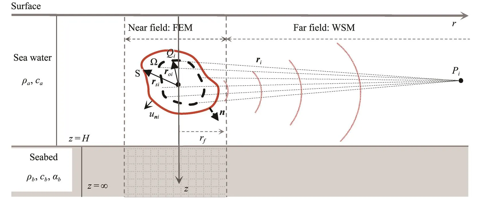
Fig.1 Schematic diagram of the wave superposition method in shallow water.

2.1 Wave Superposition Theory in Shallow Water

WSM is a computational method derived from the Hel- mholtz boundary integral (Koopmann,1989) and is suitable for calculating acoustic fields of arbitrarily shaped radiators in complex fluid environments by adjusting the GF (Miller, 1991). The sound pressureon Scan be ex- pressed by the following integral formula:

whereis the outer normal vector;is the distance vec- tor betweenQandP;andare the distances from the center of the structure to a point on S and Ω, respectively; andis the GF corresponding to the fluid environment.

In shallow water, the GF needs to satisfy the following Helmholtz equation:

The GF is obtained by solving the above equation, and different sound propagation models are derived using dif- ferent mathematical strategies. Each model has its certain applicability. In this method, the solutions for the source strength and sound field are involved in near- and far-field problems, respectively. Here, we adopt the rigorous ISM and NM to solve the near- and far-field GFs, respectively, which are discussed in detail in Subsection 2.3.

Appling the linear Euler formula, Eq. (1) can be express- ed as the form of the normal vibration velocity:

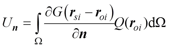
Here, the normal vibration velocity of a point on the structural surface can be constructed bysimple sources after being discretized:

whereÑis the derivative operator.

Furthermore, Eq. (4) can be expressed as the following matrix:

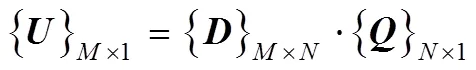
whereandare the numbers of the velocity nodes on S and simple source points on Ω, respectively.

The calculation reliability of the normal velocity matrixdirectly determines the accuracy of the WSM. Fortu- nately,is obtained by the FEM (COMSOL), which is adopted to establish a near-field model for the structural acoustic radiation affected by multi-boundary and multi-coupling systems. This part will be discussed in Subsec- tion 2.2. In Eq. (5),is the sound transfer matrix, which is defined as=Ñ(|−0|) and obtained by configur- ing the internal simple sources.

Thus, the source strength matrixcan be calculated by the identifiedandas follows:

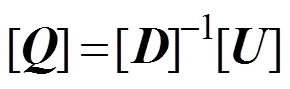
where []−1is the Moore-Penrose inverse matrix solved by the singular-value decomposition.

The sound pressure at a field point can be expressed as the following equation:

whereis a coefficient matrix and is defined as=(|−|).

The structural acoustic radiation is generally focused on the sound pressure level (SPL):

whereref=1×10−6Pa is the reference sound pressure in water.

2.2 Near-Field and Low-Frequency FEM Model

The first key step of the FE/WSM scheme is to obtain the vibration velocity on the structure surface, and the structural vibration characteristics in shallow water are only related to the boundary reflection sound in the near field. For a low-frequency acoustic problem, the amount of element meshing is relatively acceptable, so the FEM can be adapted to establish a near-field and low-frequency model for the acoustic radiation affected by the complex coupling systems. Thus, the calculated vibration velocity on the wetted structure surface is used as the input in the WSM to calculate the source strengths and acoustic radia- tion. As shown in Fig.2(a), Ωis the fluid medium do- main; Ωis the acoustic non-reflective layer,, the per- fectly matched layer (PML) domain with widthPML; and the inner and outer boundaries of the PML are Γand Γ, respectively. Γis the FSI boundary, and Γand Γare the interaction boundaries between the sound field and the surface and the seabed, respectively. According to the cor- responding boundary condition of each domain, the cou- pling equations of the structure-fluid, structure-sound, and sound-boundary are established, respectively.

The FEM formulation is derived for the acoustic fluid using the Helmholtz equation, which is based on the as- sumption that the fluid is inviscid and irrotational. More- over, by applying the weight function and Green theorem, an acoustic FEM equation can be drawn (Marburg and Nolte, 2008):

where {} is the acoustic excitation;,, andare the mass matrix, stiffness matrix, and damping matrix, respec- tively; and subscriptis the acoustic system in the fluid.

Similarly, the finite element formulation for the struc- turaldomain can be expressed as

where,, andare the mass matrix, stiffness matrix, and damping matrix, respectively, of the unconstrained part of the structural meshing, and {} is the excitation load on the node.

As shown in Fig.2(b), the first boundary condition will be satisfied on the FSI boundary (Γ) between the fluid andstructural domains, where the normal displacement (u) on the structure surface is equal to that (u) of the external fluid domain.

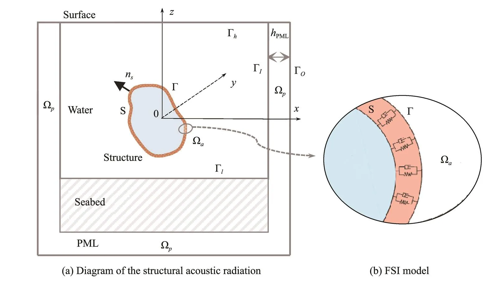
Fig.2 FEM model of the acoustic radiation in Pekeris waveguides.

whereNcontains the finite element shape functions for the structural domain S.

The second continuity condition in pressure is

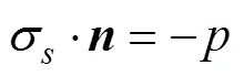
whereσis the stresses of the isotropic structure.

By substituting Eqs. (9) and (10) in Eqs. (11) and (12), the FSI problem can be described as follows:

whereandare the coupling loads of the structure and fluid domain, respectively;andare the coupling stiffness matrix and mass matrix, respectively; andT=−0T.

Theoretically, the wave equation can be converted into a PML control equation of the absorption layer by adding the absorption coefficient in the frequency domain, which can be written as follows:

whereσis the absorption coefficient in the PML andpis the sound pressure amplitude.

The PML is presented to absorb the acoustic energy so that there is no reflected sound. Furthermore, the thicknessof the PML must be greater than one-fifteenth of the maxi- mum wavelength.

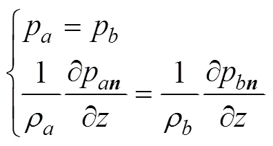
The surface boundary of the Pekeris waveguide is usu- ally modeled as the Dirichlet boundary,, the pressure- release boundary. Thus, the boundary conditions can be written as

The seabed is generally regarded as a semi-infinite liquid bottom, where the sound pressure and normal vibration velocity are equal.

The structural vibration induces the surrounding fluid through the FSI system defined in Eq. (13). Then, the fluid medium produces compression and extension motions, causing the propagation of the sound field. Furthermore, the sound propagation needs to meet specific boundary conditions,, the upper surface needs to meet the Diri- chlet boundary in Eq. (15), the lower boundary should fulfill the liquid continuous condition in Eq. (16), and the surrounding boundary should be an infinite space, which is simulated by the PML shown in Eq. (14). In addition, to avoid the disadvantages and reduce the computational cost in near-field FEM models, vibration velocities should be obtained by placing an array of sensors on the struc- tural surface in practical applications.

2.3 Near-to-Far Field Sound Propagation Models

The calculations for the source strength solution in Eq. (6) and the sound field in Eq. (7) are involved in the near- and far-field problems, respectively. Accordingly, in this subsection, the ISM and NM are adopted to improve the WSM accuracy in near-to-far-field calculations.

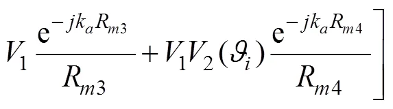
The traditional ISM is based on the ray theory, and the ideal upper and lower boundaries in the homogeneous waveguide are considered by the image sources. Fig.3 shows the contributions of a physical source and the first three image sources to the received sound field. The re- maining terms are obtained through successive imaging of the sources to yield the ray expansion for the total field:

The reflection coefficients of plane waves with various incident angles can be written as

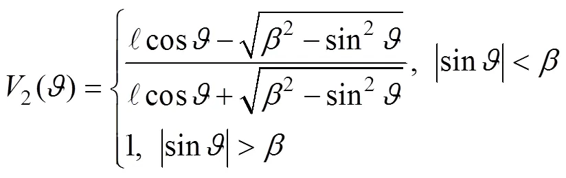
The traditional ISM described in Eq. (17) is applicable for perfectly reflecting boundaries or the low-sound-speed seabed in high frequency (Brekhovskikh, 1980), where the constant reflection coefficients of the plane waves are constant. However, for other seabeds,2is angle de- pendent, and the difficulty of the reflection problem of a spherical wave on a plane interface will occur due to the difference between the symmetries of the wave and the boundary form. Therefore, it is essential to make the wave- form and reflection coefficient consistent. In this rigorous ISM, the solution to the problem requires the decomposi- tion of spherical waves into plane waves with various an- gles:

Fig.3 Schematic diagram of the rigorous ISM for GFs in shallow water.

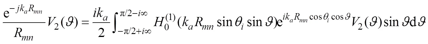
The reflected spherical wave is decomposed into the reflected plane wave by Eq. (19), which can be solved by the steepest descents, an asymptotic expansion for the Hankel function (Westwood, 1989). Then, by substituting Eq. (19) into Eq. (17), the near-field GF can be efficiently solved by this rigorous ISM, which can achieve good ac- curacy over the whole distance range and is highly adapt- able to seabed and frequencies.

The seabed area is covered with a layer of non-con- densable solid materials, which are deposited from several rivers. Thus, it is reasonable to simulate the seabed sedi- ment as a liquid domain. Furthermore, attenuation becomesa significant loss factor for long-distance propagation. Here, we describe the sound attenuation effect with the complex sound speed as follows:

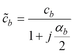
whereis the absorption coefficient in the fluid seabed and measured in the form of a wavelength,,α(dBλ−1), which is given by the expression asα(dBλ−1)=27.3α.

The NM of the far-field propagation model is derived bythe separation of variables, and Eq. (2) can be rewritten into cylindrical coordinates in the depth and distance di- rections as follows:

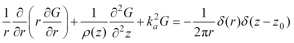
where0is the depth of the source position,0−z,is the field point position, and() and(−0) are the Dirac functions in the horizontal distance and depth di- rections, respectively.

The above non-homogeneous equation is solved by the separation of variables with the form of the(,)=()(), and the sound field can be described as the sum of the NMs:

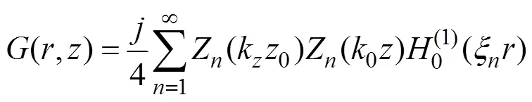
whereis the imaginary unit of the complex number;Z(kz) is the eigenfunction, which is determined by the upper and lower boundaries; andξandkare the eigenvalues of the horizontal and vertical directions, respectively.

The general solution for the eigenfunctions is

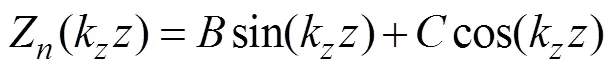
The upper surface of the ocean is the Dirichlet condition, which is defined as follows:

The acoustic boundary equation for the liquid seabed can be defined as

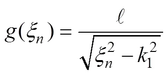
where(ξ) is determined by the identified seabed para- meters, and the relationship with the interface reflection coefficient2can also be established through the follow- ing equation (Katsnelson, 2012):

Similarly, we describe the sound attenuation effect with the complex wavenumber as follows:

By substituting Eq. (23) into Eqs. (24) and (25), we ob- tain

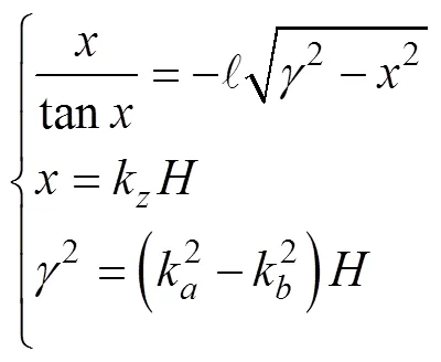
The far-field GF based on the NM can be obtained ac- cording to the eigenvalue Eq. (29), which is a transcen- dental equation in the complex domain and cannot be solved accurately using conventional numerical methods. Here, a mature calculation program KRAKENC (Porter and Reiss, 1984) is adopted to exactly find complex ei- genvalues in a complex plane (Porter and Reiss, 1985).

3 Theoretical Model Verification

The FE/WSM calculation procedure for predicting the acoustic radiation of the arbitrary radiator in Pekeris wave- guides is mainly divided into three steps:

1) A near-field acoustic radiation model is established by the FEM, and a complex coupling system is solved to ob- tain the normal velocity matrixon the structural wetted surface.

2) Simple sources are optimally configured inside the elastic radiator, where the source strength matrixis solved by combining Eqs. (6) and (17) in the near field.

3) The sound field matrixgenerated by each simple source at a receiver is calculated using Eqs. (7) and (22) in the far field.

Thus, an important factor that determines the accuracy of this method is the source strength solution, which is decided by the vibration velocity matrix, sound source con- figuration, and near-to-far-field GFs. Drawing on the pre- vious remarkable work, in this study, the vibration veloc- ity solution in the near-field FEM model is established by the software COMSOL (Piacsek and Muehleisen, 2014; Jiang, 2018), and the optimal configuration of the simple sources (Miller, 1991) can be effectively guaran- teed. However, the latter GF has its adaptability and ac- curacy to frequency, distance, and environment, which will significantly affect the accuracy and efficiency of the FE/WSM calculation.

In this section, the sound field of a point source in Pe- keris waveguides with the lossy seabed is performed as the first numerical experiment, which is adopted to verify the GFs in the near-to-far-field propagation models. SPLs with different frequencies are calculated using the near-field ISM and far-field NM models and compared with theoretical solutions based on WI (Schmidt and Glattetre, 1985). Then, the acoustic radiation models of the excited elastic spherical and cylindrical shells in the same Pekeris waveguide are served as the verification examples for the proposed FE/WSM. The acoustic radiation fields are cal- culated and compared with the FEM solutionsCOM- SOL. Finally, a comparative analysis of the execution time is presented. These numerical models illustrate the accu- racy and efficiency of the proposed FE/WSM for com- puting the 3D acoustic radiation of an elastic structure in the Pekeris waveguide.

3.1 Validation of Results with Near-to-Far-Field Models

A typical sound propagation model in a Pekeris wave- guide is established to verify the GFs, which are described by the rigorous ISM and NM. As depicted in Fig.4, which shows a point source with 15m depth, the upper surface is the released pressure, the depth of homogeneous water is 30m, and the density and sound speed areρ=1024kgm−3andc=1500ms−1, respectively. The density and sound speed of the liquid seabed areρ=2000kgm−3andc=1800ms−1, respectively, with a sound absorption of 0.5dBλ−1. The depth of each receiver is 15m, and the horizontal interval is 1m.

The relationship between the reflection coefficient2and incident angleis calculated by Eq. (18), which is shown in Fig.5. When the liquid seabed has no sound absorption, there is an incident angle (, the critical angle=arcsin(c/c)≈56˚), where the sound field on the in- terface appears to be a total reflection, and the reflection coefficient is a constant of 1. By contrast, when the me- dium contains acoustic absorption withα=0.0dBλ−1,α=1.0dBλ−1, andα=2.0dBλ−1, the reflection coefficient varies with the angle of incidence. In the range of 0˚–10˚, within which the reflection coefficient can all be approxi- mated as 0.41, the GF can be described by the spherical wave directly multiplied by a constant reflection coeffi- cient in the near range of≤0.18(z+). However, the ap- plicable distance is too short (generally a few meters), which is not competent for describing computational near-field acoustic problems, such as the source strength solu- tion and near-field sound field calculation. Furthermore, the traditional ISM is generally applicable for perfectly reflecting boundaries or low-sound-speed seabeds and in boundaries whose reflection coefficient is unity or does not depend on the incident angle in the limited angle range. Thus, it is necessary to strictly observe the wave acoustics method to establish the interaction mechanism of the near-field spherical wave and interface. Accordingly, a near-field GF can be induced by this rigorous ISM described in Eq. (19).

Fig.4 Typical sound propagation of a point source in the Pekeris waveguide.

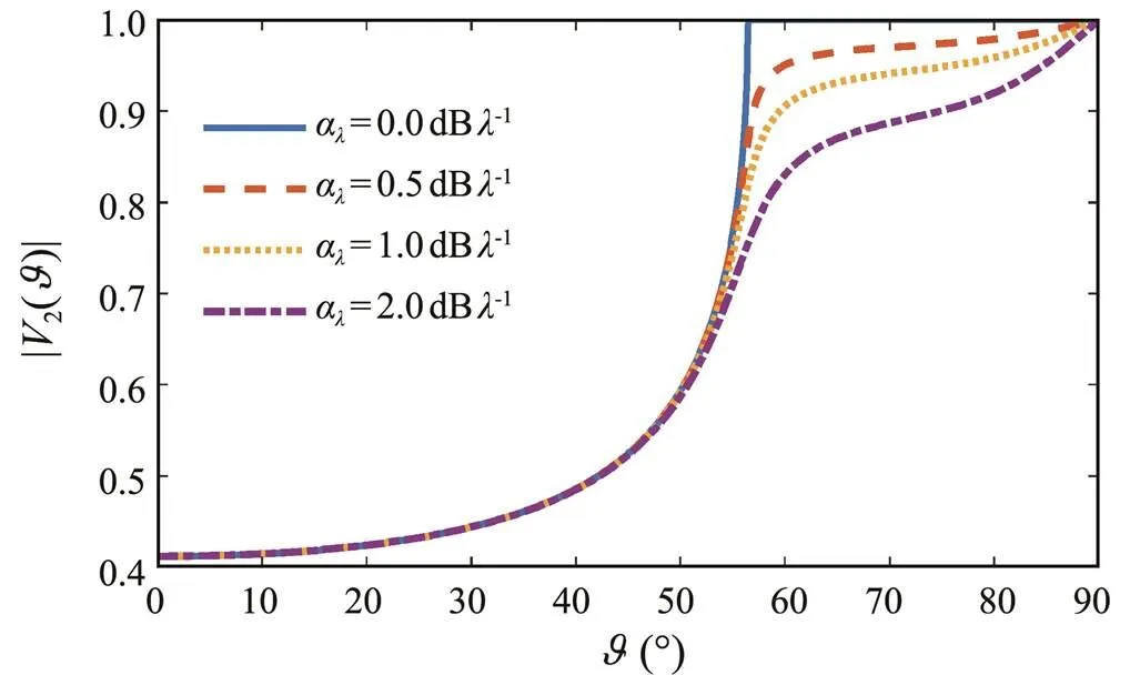
Fig.5 Reflection coefficientsversus incident angles for dif- ferent absorptions.

To make the sound propagate over long distances rather than rapidly attenuate, the frequencies in the Pekeris wave- guide can be above the cutoff frequencyfgiven by

The propagation frequencies associated with the first 6-order NMs are shown in Table 1. If the frequency is lower than the first-order frequency,,1=22.60Hz, then the sound will rapidly decay with the distance and cannot travel far away. The accuracies of the rigorous ISM and complex NM for the near- and far-field acoustic problems are fully compared, respectively. The frequencies are 50, 100, 200, and 400Hz, which are selected according to geometric sequences.

Table 1 Propagation frequencies of first six-order NMs

The SPLs of a point source in this waveguide are cal- culated by adopting the rigorous ISM and complex NM. The results are compared with the theoretical solutions accurately calculated by the WI, whose range is 0–2000m. As shown in Fig.6, the results between the ISM and theoretical WI solutions are in good agreement in the near field, and the NM achieves the same performance in the far field. The incident spherical wave of a point source on the fluid-fluid surface will produce plane waves and non-uniform plane waves (, leakage modes), which are not considered in the NM solution. Thus, the NM is an ap- proximate solution and has a certain difference in the near field, which is not suitable for the near-field problem. However, these higher-order leakage modes decay accord- ing to the 1/2with distance and completely attenuate with- in two to three wavelengths (Brekhovskikh, 1980). There- fore, the NM with only a few orders can be used to effec- tively describe the sound propagation and achieve a good performance after reaching a certain distance, which is suitable for far-field sound field problems. The rigorous ISM considers the upper and lower boundaries through the image sources generated by the upper and lower bounda- ries. Furthermore, it observes the wave acoustic method and establishes the interaction mechanism of the near-field spherical wave and interface through Eq. (22). Thus, the rigorous ISM is an exact solution and adaptable to seabed parameters and frequencies, which can handle near-field acoustic problems.

Fig.6 Sound field comparison between the near- to far-field model and theoretical solution.

Due to the distances between the simple sources and because structural surface nodes are within a few wave- lengths, the strength solution is considered a near-field acoustic problem. On the contrary, the structural acoustic radiation in the waveguide is generally focused on sound propagation with several kilometers, which is a far-field problem. Considering the computational accuracy and effi-ciency of the proposed FE/WSM scheme, we use the rig- orous ISM and NM to solve the near-field source strength solution and far-field sound field calculation, respectively.

3.2 Acoustic Radiation Prediction of an Elastic Spherical Shell

To verify the reliability of the proposed method for pre- dicting the acoustic radiation of an elastic radiator in the waveguide, a schematic diagram of the FE/WSM model of an elastic spherical shell, which is excited by a har- monic point excitation, is shown in Fig.7(a). We consider the case where the spherical shell, excitation configura- tion, and fluid are all in good symmetry. The 3D elastic spherical shell can be converted into a 2D acoustic radia- tion model by the axisymmetric coordinates to reduce the FEM calculation cost. Fig.7(b) shows an FEM meshing model. The mesh size of the fluid domain is one-sixth of the wavelength, and the mesh sizes of the elastic spherical surface and nearby fluid are refined. The upper and lower surfaces are modeled as the Dirichlet boundary and liquid lossy seabed, respectively. The infinity boundaries in the fluid and seabed domains are simulated with multiple PML domains so that there is no reflection sound. The center of the shell is located at a depth of 15m, and the harmonic point excitation isF=1N, which is vertically applied at the top of the spherical shell with a radius of 3m. The thickness is 0.01m, the material used is steel (type=AISI 4340, densityρ=7850kgm−3, Young’s modulusE=2×1011Pa, and Poisson’s ratiou=0.33).

Fig.7 Acoustic radiation model of a spherical shell in the Pekeris waveguide.

In the calculation process of the 3D FE/WSM, the 2D FEM result needs to be converted into a 3D problem, and the normal vibration velocities on the 3D spherical shell surface are extracted. Then, an array of simple sources is configured reasonably inside the radiator to improve ac- curacy and efficiency. In the instructive work performed by Koopmann(1989) and Miller (1991), the num- bers of node points on the pulsating sphere and fictitious surface were set as 290 and 192, respectively. The ficti- tious surface Ω,with radiusr=1.5m, is a spherical sur- face with the same shape as the radiator surface S. To reduce the computational cost and implementation work- load, the easily accessible SPL-curve is presented to de- scribe the performance of the method for computing the far-field acoustic radiation of large radiators in shallow water. The frequencies of all curves are selected accord- ing to geometric sequences (50, 100, 200, and 400Hz), the horizontal interval of each receiver is 1m, and the depthis 15m. Other environmental parameters and receiver selec- tions are the same as those of the above verification model.

The SPL-comparisons between the FE/WSM and FEM for a 3D elastic spherical shell in the Pekeris waveguide are presented in Fig.8. The blue solid and red dashed lines represent the FEM and FE/WSM solutions. A good agree- ment between the two methods is achieved. Particularly for low-frequency acoustic radiation calculations, both me- thods are completely consistent over the entire calculated distance at each frequency. In the near field, a certain de- viation problem is introduced using the finite number of velocity nodes on the structure surface to describe the com- plex vibration shape, and various internal simple sources are placed uniformly to be equivalent to the acoustic field of the structure. Moreover, the FE/WSM does not take into account the shading effect of the physical structure on the near-field sound field, resulting in some near-field differ- ences with the more practical FEM solutions. However, the overall trend of the acoustic radiation is consistent be- cause this shading effect will rapidly disappear.

Fig.8 SPL comparison of the elastic spherical shell between the FE/WSM and FEM.

3.3 3D Acoustic Radiation of the Asymmetric Cylindrical Shell

Further validation is performed to show the accuracy and efficiency of computing the 3D problem in an asymmetric condition. Fig.9 presents the 3D acoustic field of a slen- der cylindrical shell in the Pekeris waveguide. As shown in Fig.10(a), the finite cylindrical shell, water column, and seabed are modeled by the frequency-domain FEM to ob- tain the vibration velocity in the near field, where the re- quirements for the element meshing of the near-field local model are stringent. Fig.10(b) shows a representation of the meshing model for fluid, structure, seabed, and PML. The cylindrical shell is modeled with uniform surface ele-ments with the following properties: length=10m, radius=1m, thickness=0.01m, and center depth=15m. A downward excitation force is vertically applied to the center point on the upper surface, with forceF=1N. The material properties, waveguide environment parameters, and receiver selection are the same as those in the above verification examples.

The vibration velocity on the 3D cylindrical shell sur- face is efficiently calculated by the FEM model. Here, the normal velocities of 176 nodes on the structural surface are selected as the input for source strength solutions in the WSM. Due to the vibration complexity on the structure surface in the asymmetric coordinate, simple sources with 160 points are needed, which are uniformly distributed on the fictitious surface Ω to achieve the desired calculation accuracy. The geometry shape of the surface Γ is conformal to the cylindrical surface, and the geometric size ratio is 2:1 (, the radius lengths of Γ are 0.5 and 5m).

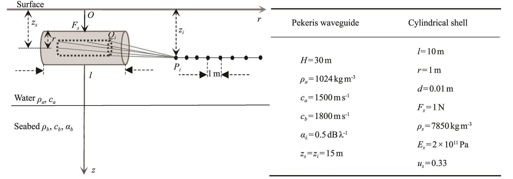
Fig.9 Schematic diagram of the structural model of the FE/WSM.

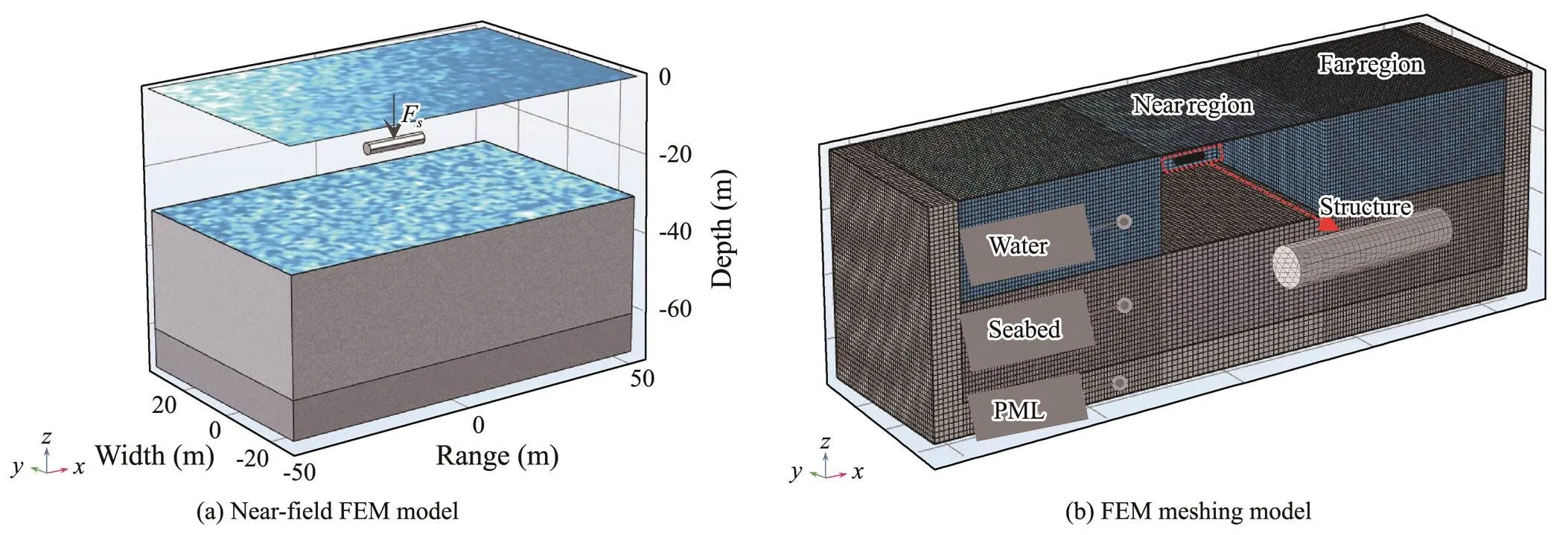
Fig.10 Acoustic radiation model of the cylindrical shell in the Pekeris waveguide.

To the best of the author’s knowledge, few analytical works have been performed on the free flexural vibration of huge finite cylindrical shells in Pekeris waveguides. Here, we attempt to adopt the FE/WSM to compute the 3D acoustic radiation in low frequencies and compare it with the standard FEM results in a long-distance range,, 0–1000m. As shown in Fig.11, the SPL in theplane is presented from the 3D FEM model as a comparison of the results calculated by the FE/WSM. Clearly, the sound field distribution of the cylindrical shell calculated by both methods is consistent, and good performance is also achieved for other computable frequencies of the far-field FEM results. For example, when=50Hz, the wave wave- length is 30m. Only a complete NM appears in the depth direction of the radiated sound field in Figs.11(a)–(b), and two full NMs appear when the frequency increases to 100Hz in Figs.11(c)–(d). The consistency of the calculation results for both methods can be obtained in other planes and directions.

Because the far-field 3D FEM results are limited by the calculated capability of the platform and reduce the im- plementation workload, SPL-curves at 50 and 100Hz are selected according to geometric sequences. The SPL-results of the FE/WSM and FEM are compared in detail to show the suitability of the method for low-frequency acoustic problems. Fig.12 demonstrates a comparison for an array of receivers with a depth of 15m, and a good agreement between both methods can be achieved in the total range except that there are few deviations in the short-distance range. For example, a maximum error of 4dB appears at 8m when=50Hz (Fig.12(a)), and a maximum peak error of 8dB appears at 35m when=100Hz (Fig.12(b)). Compared with the axisymmetric spherical shell, the vibroacoustics of an asymmetric elastic cylindrical shell are more complicated, and this method uses the finite vibration nodes and simple internal sources to separately describe the vibration and acoustic characteristics of the continuous structure. This processing is a semi-analytical numerical method and has inevitable structural discretiza- tion and acoustic equivalence errors, introducing small ap- proximation errors (generally a few percent) into the whole calculation. The FE/WSM does not take into account the shading effects of the physical structure on the near-field acoustic radiation, introducing computational deviations between the FE/WSM and FEM solutions into the near field. However, these geometry shading effects will rap- idly disappear and do not have a significant impact on the accuracy of the acoustic calculation. Thus, a good agree- ment between both methods (FEM and FEM/WSM) can be achieved in the whole range, and these computational re- sults enable this method to be accepted for investigating the structural acoustic radiation in the ocean.

Fig.11 SPL comparison of the elastic cylindrical shell in the xz plane.

Fig.12 SPL comparison of the elastic cylindrical shell between the FE/WSM and FEM.

3.4 Efficiency of the Proposed Method for 3D Acoustic Calculations

To show the efficiency of the proposed method for the 3D ocean acoustic field, an execution time test of differ- ent distances () and frequencies () is conducted. A vali- dation example,, an elastic cylindrical shell excited by a point force in the Pekeris waveguide, is used as a test model. The 3D FEM model is established by COMSOL, as shown in Fig.10, and the computational program is compiled with MATLAB. The interval between receivers in this method is the same as the FEM mesh size,, one-sixth of the wavelength, and the shape of the fluid domain for the near-field FEM model in the FE/WSM is a cylinder with a radius of two to three wavelengths. All calculations are run on Dell Precision 5820 Tower, with Intel(R) W-2133 3.60GHz and 96GB RAM.

Of note, NOF is the number of freedom of the FEM mesh, andis the execution time ratio between the FEM and proposed method, that is,=1:2, we assume that the calculation time is infinity (∞) when the NOF is increased beyond the computational capability of the 5820 Tower.

The execution time comparison of both methods in dif- ferent frequencies and distance ranges is presented in Ta- ble 2. First, the calculation efficiencies at different fre- quencies are analyzed independently to keep the distance constant (0–0.5km). Because the execution time of the computational method is mainly spent in step 1,, a near-field model is established by the FEM, the NOF is posi- tively correlated with the frequency. For example, the execution time ratio drops from 18 to 12 times when the frequency increases from 50 to 100Hz. For the latter case, where the main calculation time of the near-field FEM model with an NOF of 4.02×105(step 1) is approximately20.73min, the required solution time for the source strength (step 2) and sound field (step 3) in the WSM is approxi- mately 4.49min. Thus, the total time for a 3D acoustic problem is approximately 25.22min (, 0.42h), which is five times more efficient than the 3D FEM model, which costs approximately 5.12h to complete the calcula- tion. In addition, the efficiency advantage of the presented method gradually emerges with the increase in frequency because the FEM mesh needs to be more refined as the frequency increases in the whole calculated domain, re- sulting in a significant increase in the NOF, and requires more time to finish the numerical computation. When the calculated frequency is higher than 150Hz, the NOF is greater than 14.97×106, causing the computer memory leak problem in this hardware and failure to complete the cal- culation. However, the FE/WSM can be competent for the calculation within a few hours, greatly improving the com- putational efficiency in the low-frequency domain.

Table 2 Comparison of the execution time test results between the FEM and FE/WSM

Simultaneously, the time test results in different dis- tance ranges are given, and the constant frequency is 100Hz. The computational advantage of this method is not notable in the close range, and its efficiency is only sev- eral times (ratio=12:1) higher than that of the FEM in a calculation range of 0–0.5km. Moreover, at different distances, step 1 of the near-field FEM and step 2 of the source intensity calculation time remain constant (approxi- mately 21.00min), the difference in the execution time is mainly consumed in step 3,, sound field calculation. Because the computation time for each sound field point is the same, the calculated time in this step linearly in- creases with the field points, and the efficiency advantage is relatively small (approximately 4min) for the sound field in this range (0–0.5km). When the range is 0–5km, the NOF of an FEM solution reaches 41.17×106, and the sound field calculation becomes extremely limited by the memory leak problem and fails to complete the computa- tion. However, this sound field can be quickly calculated by the FE/WSM within 1.02h, which can greatly improve the efficiency of long-distance calculations. Moreover, the computation cost and accuracy are independent of the calculation distance and field point interval.

Therefore, this method can reduce the calculation cost by at least ten times than the FEM and greatly improve the efficiency of the 3D sound field radiated from huge structures in shallow water, especially for long-distance and low-frequency problems. It also has significant po- tential for acoustic radiation prediction, sound measure- ment, and target location in practical engineering.

4 Conclusions

In this study, we propose an effective and accurate semi-analytical FE/WSM to calculate the 3D acoustic radiation for arbitrary-shaped structures in the ocean. This FE/WSM is modeled by the more widely used Pekeris waveguide rather than an ideal environment, and influences of the upper surface and lossy seabed on the vibroacoustic char- acteristics are considered. The theoretical model consists of the near-field FEM and WSM, which are respectively presented for discrete structures and far-field sound cal- culation. The calculation procedure is mainly divided into three steps: First, in a near-field FEM solution, a 3D acous- tic radiation model is established by the FEM, and the vibroacoustic information on the structure surface is ob- tained conveniently. Second, in the near-to-far-field propa-gation model, the GFs in the Pekeris waveguide are solved by the rigorous ISM and NM to accurately solve near- and far-field problems, respectively. Third, in the WSM calculation, an array of equivalent simple sources is opti- mally configured inside an elastic radiator, source strengths are solved by combining the structural surface velocity the near-field GF, and a scheme adopting the superposition of acoustic fields generated by an array of simple sources is adopted to predict the total sound pressures, which can be equivalent to the acoustic radiation of the radiator.

A new near-to-far-field method is presented for the low-frequency acoustic radiation of an elastic structure in the Pekeris waveguide. This model considers the advan- tages of the FEM, which is a powerful numerical approach for calculating near-field and acoustic radiations. More- over, the WSM can be easily implemented in the far-field acoustic radiation by optimizing simple source configura- tions and combing adjustable GFs. A typical point source in the Pekeris waveguide is presented to verify near-to-far-field GFs, and the results are compared to those from a theoretical WI. We found that the rigorous ISM based on the spherical wave superposition is an exact solution and is adaptable to seabed parameters and frequencies, which can effectively handle near-field acoustic problems in the proposed theoretical model. Moreover, the NM has po- tential in the far-field sound field, thus proving that near- and far-field GFs are an accurate and reliable concept. The verification models of the sound field from huge elastic spherical and cylindrical shells in the Pekeris waveguide are established, where only 192 and 160 simple sources are respectively required and highly accurate results are calculated. Comparing the FEM solutions calculatedCOMSOL, we deem that this method can provide a better computational performance and reduce the calculation cost by tens to hundreds of times than the FEM, especially for long-distance problems. Furthermore, it overcomes the dif- ficulties of previous methods that are limited to structural shapes and complex oceans and can lay a groundwork for the integrated calculation of SSI, acoustic radiation, and sound propagation for radiators in ocean-acoustic envi- ronments.

Furthermore, we present a computationally adaptable scheme to discretize continuous radiators and analytically calculate the sound field in complex oceans. Compared to traditional methods, this method is independent of the acoustic structure size, frequency, and calculation distance. Moreover, it can not only analyze the SSI vibration and acoustic radiation in the near field but also efficiently calculate the radiation (scattering) sound field of arbi- trary-shaped radiators (scatters) and solve these problems with low calculation cost and succinct calculation proce- dures. These features, together with increased computa- tional power, should make the proposed method attractive to acoustic stealth design, sound measurement, and target location, considering practical ocean environments in the foreseeable future.

Acknowledgements

The authors are grateful for the discussions with their colleagues that led to the development of this study. In particular, this work is financially supported by the Na- tional Key Research and Development Plan of China (No. 2016YFC1401203) and the National Natural Science Foundation of China (Nos. 42006168 and 11404079).

Bai, Z. G., Wu, W. W., Zuo, C. K., Zhang, F., and Xiong, C. X., 2014. Sound radiation and spread characteristics of cylindri- cal shell in finite depth water., Z1: 178-190 (in Chinese with English abstract).

Ballard, M. S., 2019. Three-dimensional acoustic propagation effects induced by the sea ice canopy, 146 (4): EL364-EL368.

Brekhovskikh, L. M., 1980..2nd edi- tion. Academic Press, New York, 228-234.

Cockrell, K. L., and Schmidt, H., 2010. A relationship between the waveguide invariant and wavenumber integration., 128 (1): EL63-EL68.

Collis, J. M., Frank, S. D., Metzler, A. M., and Preston, K. S., 2016. Elastic parabolic equation and normal mode solutions for seismo-acoustic propagation in underwater environments with ice covers., 139 (5): 2672-2682.

Fahnline, J. B., and Koopmann, G. H., 1991. A numerical solutionfor the general radiation problem based on the combined meth- ods of superposition and singular-value decomposition., 90 (5): 2808-2819.

Irena, L., and Henrik, S., 2006. Subcritical scattering from buried elastic shells., 120 (6): 3566-3583.

Jensen, F. B., Kuperman, W. A., Porter, M. B., Schmidt, H., and Bartram, J. F., 2011.Springer, New York, 103-105.

Jiang, L. W., Zou, M. S., Huang, H., and Feng, X. L., 2018. Inte- grated calculation method of acoustic radiation and propaga- tion for floating bodies in shallow water.,143 (5): EL430-EL436.

Jiang, L. W., Zou, M. S., Liu, S. X., and Huang, H., 2020. Cal- culation method of acoustic radiation for floating bodies in shallow sea considering complex ocean acoustic environments., 476: 115330.

Junger, M. C., and Feit, D., 1986.MIT Press, Cambridge, 235-251.

Katsnelson, B., Petnikov, V., and Lynch, J., 2012.Springer, New York, 79-92.

Klaseboer, E., Sepehrirahnama, S., and Chan, D., 2017. Space-time domain solutions of the wave equation by a non-singular boundary integral method and Fourier transform., 142 (2): 697-707.

Koopmann, G. H., Song, L., and Fahnline, J., 1989. A method for computing acoustic fields based on the principle of wave su- perposition., 86 (6): 2433-2438.

Liu, R. Y., and Li, Z. L., 2019. Effects of rough surface on sound propagation in shallow water., 28 (1): 423-430.

Ma, Z., Cheng, Y., Zhai, G. J., and Ou, J. P., 2015. Hydroelastic analysis of a very large floating structure edged with a pair of submerged horizontal plates., 14: 228-236.

Marburg, S., and Nolte, B., 2008.. Springer, Berlin Heidelberg, 24-40.

Miller, R. D., 1991. A comparison between the boundary element method and the wave superposition approach for the analysis of the scattered fields from rigid bodies and elastic shells., 89 (5): 2185-2196.

Oğuz, H. N., 1996, Emission of sound by a semi-submerged object in shallow water.,100 (1): 252-261.

Pan, S. W., Jiang, W. K., Zhang, H. B., and Xiang, S., 2014. Mod- eling transient sound propagation over an absorbing plane by a half-space interpolated time-domain equivalent source method., 136 (4): 1744-1755.

Pang, F., Li, H., Cui, J., Du, Y., and Gao, C., 2018. Application of flügge thin shell theory to the solution of free vibration behaviors for spherical-cylindrical-spherical shell: A unified formulation., 74: 381-393.

Paul, C. E., 2003.. 3rd edition. Spon Press, New York, 94-97.

Piacsek, A. A., and Muehleisen, R. T., 2014. Using COMSOL multiphysics software to investigate advanced acoustic prob- lems.,130: 2363- 2363.

Ping, G., Chu, Z., Xu, Z., and Shen, L., 2017. A refined wideband acoustical holography based on equivalent source method., 7: 43458.

Porter, M. B., and Reiss, E. L., 1984. A numerical method for ocean acoustic normal modes., 76 (1): 244-252.

Porter, M. B., and Reiss, E. L., 1985. A numerical method for bottom interacting ocean acoustic normal modes., 77: 1760-1767.

Schmidt, H., and Glattetre, J., 1985. A fast field model for three-dimensional wave propagation in stratified environments based on the global matrix method., 78 (6): 2105-2114.

Shang, D. J., Qian, Z. W., He, Y. A., and Xiao, Y., 2018. Sound radiation of cylinder in shallow water investigated by combined wave superposition method., 67 (8): 125-138 (in Chinese with English abstract).

Wang, P., Li, T. Y., and Zhu, X., 2017. Free flexural vibration of a cylindrical shell horizontally immersed in shallow water using the wave propagation approach., 142: 280-291.

Westwood, E. K., 1989. Complex ray methods for acoustic in- teraction at a fluid-fluid interface., 85 (5): 1872-1884.

Xu, C. X., Zhang, H. G., Piao, S. C., Yang, S. E., Sun, S. P., andTang, J., 2017. Perfectly matched layer for an elastic parabolic equation model in ocean acoustics., 16 (1): 57-64.

Yang, G., Yin, J. W., Yu, Y., and Shi, Z. H., 2016. Depth classi- fication of underwater targets based on complex acoustic in- tensity of normal modes., 15 (2): 241-246.

Zhang, Y. B., Bi, C. X., Chen, X. Z., and Chen, J., 2008. Compu- tation of acoustic radiation from vibrating structures in motion., 69 (12): 1154-1160.

Zhang, Y. N., Jie, P., Chen, K. A., and Zhong, J., 2018. Sub- wavelength and quasi-perfect underwater sound absorber for multiple and broad frequency bands., 144 (2): 648-659.

Zhao, X., and Wu, S. F., 2005. Reconstruction of vibroacoustic fields in half-space by using hybrid near-field acoustical holography., 117 (2): 555-565.

Zhong, J., Zhao, H., Yang, H., Yin, J., and Wen, J., 2019. On the accuracy and optimization application of an axisymmetric sim- plified model for underwater sound absorption of anechoic coatings., 145: 104-111.

Zou, M. S., Liu, S. X., Jiang, L. W., and Huang, H., 2020. A mixed analytical-numerical method for the acoustic radiation of a spherical double shell in the ocean-acoustic environment., 199: 107040.

Zou, M. S., Wu, Y. S., and Liu, S. X., 2018. A three-dimensional sono-elastic method of ships in finite depth water with ex- perimental validation., 164: 238-247.

Zou, M. S., Wu, Y. S., Liu, Y. M., and Lin, C. G., 2013. A three-dimensional hydroelasticity theory for ship structures in acous- tic field of shallow sea., 25 (6): 929-937.

January 5, 2021;

April 1, 2021;

July 12, 2021

© Ocean University of China, Science Press and Springer-Verlag GmbH Germany 2022

. E-mail: jingsheng@tju.edu.cn

(Edited by Xie Jun)