
Useful zero friction simulations for assessing MBS codes Pascal’s formula giving wheelsets frequency for zero wheel-rail friction
2022-08-26 07:42JeanPierrePascal
Jean Pierre Pascal
Pascal Coding, Rue d’Erquy, Pleneuf-Val-Andre F-22370, France
Keywords:Unsuspended wheelsets Klingel formula Rigid contact Harmonic oscillation Multi body system railway codes Code validation
ABSTRACT Present study provides a simple analytical formula, the “Klingel-like formula” or “Pascal’s Formula” that can be used as a reference to test some results of existing railway codes and specifically those using rigid contact. It develops properly the 3D Newton-Euler equations governing the 6 degrees of freedom (DoF) of unsuspended loaded wheelsets in case of zero wheel-rail friction and constant conicity. Thus, by solving numerically these equations, we got pendulum like harmonic oscillations of which the calculated angular frequency is used for assessing the accuracy of the proposed formula so that it can in turn be used as a fast practical target for testing multi-body system (MBS) railway codes. Due to the harmonic property of these pendulum-like oscillations, the square ω 2 of their angular frequency can be made in the form of a ratio K/M where K depends on the wheelset geometry and load and M on its inertia. Information on K and M are useful to understand wheelsets behavior. The analytical formula is derived from the first order writing of full trigonometric Newton-Euler equations by setting zero elastic wheel-rail penetration and by assuming small displacements. Full trigonometric equations are numerically solved to assess that the formula provides ω 2 inside a 1% accuracy for usual wheelsets dimensions. By decreasing the conicity down to 1 × 10 -4 rad, the relative formula accuracy is under 3 × 10 -5 . In order to test the formula reliability for rigid contact formulations, the stiffness of elastic contacts can be increased up to practical rigidity (Hertz stiffness × 10 0 0).
Klingel’s formula calculates the angular frequency of wheelsets but is not fitted for slippery cases: Provided sufficient wheel-rail friction and under some initial perturbation, an isolated wheelset running over a straight railway track will be hunting quasisinusoidally with wavelength and frequency properly predicted by Klingel’s formula,ω2=V2[2γ/(RE)], that Klingel derived (1883)from the assumption that there is no wheel-rail slippage [1–3] .This assumption works in real life because, even if there is always some wheel-rail slip, it is very small when wheelsets are not braking. Thus, up to now, Klingel’s formula was never contradicted by practitioners [4] . This note shows that for the theoretical case with zero wheel-rail friction, railway wheelsets would oscillate, pendulum like, from right to left of the track independently of the forward speed with a well defined frequency,ω, that all railway dynamical codes can calculate accurately just by settingμ= 0 in their model of unsuspended wheelsets. But, since Klingel’s formula does not apply for cases of zero friction, a new Klingel’s formula is advisable to provide a referenceωvalue. Thus,although zero friction cases do not interest practitioners, their study is enlightening for railway engineers and code developers. Hence, without enough friction coefficient, the sole wheel-rail forces are normal to the contacts, wheel-rail slippage is free to develop, Klingel’s formula does not apply and a new formula is needed.
A new “Klingel-like formula” can help assessing multi-body system (MBS) codes: due to the specificity of wheelset/track geometry, writing properly railway dynamical codes deals with many trigonometric equations which aim at calculating bodies accelerations in order to integrate them numerically. As of wheelsets,programmers choose between rigid or elastic wheel/rail contact formulations. A priori, avoiding the burden of contact itself, geometry of rigid contacts seems easier than elastic contacts and leading to less time consuming for numerical integrations. However, with rigid contact, lateral, vertical and roll displacements of the wheelset are rigidly linked so as to be reduced to only one degree of freedom of which calculating the exact acceleration and then integrating it as function of time, using reasonable time steps, is not straightforward since there exist no explicit equation to calculate contact forces in this case [5] ; indeed,results of commercial codes using rigid contact formulations recently revealed questionable when confronted to elastic formulations [6] . Each programmer has to find clever iterations trade-offs to solve these issues of which it is not easy to verify the validity when, at the end of the day, simulations results are dominated by creepage forces. Happily, in the frame of MBS coding, programming elastic contacts allows to separate the six wheelset degrees of freedom (DoFs) to write six explicit independent Newton-Euler equations whilst analytical Hertz equations can be used safely to calculate wheel/rail normal contact forces from geometrically calculated wheel-rail interpenetrations. Setting zero friction eliminates the burden of creepage forces [7] and using constant conicity eliminates complications as to calculating wheel profiles curvatures. By increasing the contact stiffness it is possible to come very close to the rigid proper solution (up to the point of avoiding numerical instabilities of the solver). However, all dynamical Newton-Euler equations remain valid and their solving result in wheelset oscillations. Any approximation in equations development would be revealed by approximative frequency results whenever a reliable frequency target is provided. The proposed test is founded on using the code to be tested to calculate the frequency of small harmonic oscillations of unsuspended wheelsets occurring when contacts develop inside the constant conicity part of wheel treads and when wheel/rail friction is set at zero. The frequency calculated by the code is then compared to a target frequency. A “Klingel-like formula” could be here formulated to provide the target frequency,then, a numerical “target-code”, solving the full system of equations, was used to assess its reliability. The numerical ‘target- code’is here developed and details are disclosed so as being able to calculate precisely the oscillations of any given wheelset geometries and forward velocities including rotational moments. The choice of the integration time step and the stability study of this numerical calculation are provided in Ref. [8] . However, using a low forward velocity, such as 5 or 10 m/s, associated to a low pitch velocity, we have shown that rotational effects on the wheelset oscillation frequency can be neglected and that the analytical “Klingellike formula” gives a good approximation (<1%) of the square of the frequency as function of the wheelset geometry, inertia and gravity. In the railway population, a 1% accuracy of the measurable results is considered as a perfect target in the very un-perfect real world. When comparing the target-frequency to that coming out of simulations of the tested code, either the code could be validated or not whether large frequency discrepancies (>5%) would characterize too large coding simplifications or even inadvertent flaws.
In a previous publication [9] we have studied the behavior of unsuspended wheelsets with respect to speed and initial conditions. As of wheelsets using nonconformal wheel/rail pairs, meaning constant conicity wheelsets, it was found that, given a non zero friction coefficient (0.1<μ <0.5), they are always unstable whatever the speed or initial conditions. On a running wheelset, the load has two main effects, one relates to normal forces and conicity, the other, far more complicated, deals with creepage forces notably depending on the wheel-rail friction coefficient; here energy balance plays a major role. In order to separate both effects, present paper will deal with the behavior of an unsuspended wheelset with zero creepage forces (μ= 0) meaning zero damping.Such a wheelset, of which a sketch is presented in Figs. 1 and 2 ,behaves like a pendulum capable, whether excited, of oscillating about its stable equilibrium which is in the symmetrical lowest situation. The harmonic frequencyωof this pendulum does not depend on the wheelset forward speed if the wheelset pitch rotation is set at zero, then there are no gyroscopic moments and the yaw angle will stay at zero. Since in usual codes, the initial pitch velocity is automatically related to the initial forward speed through wheels radii, it would suffice to set a low initial speed whether needed to neglect gyroscopic moments.
If the squareω2could be calculated as a constant in the form:ω2=K/M, whereKdepends only on the wheelset geometry andMon its inertia, then the wheelset oscillation would be harmonic,such as its displacements will be proportional to sin(ωt) functions.Reciprocally, if the calculated oscillating displacements, as functions of time, would be found harmonic of frequencyω, then there exist a ratioK/MwhereKdepends on the wheelset geometry andMdepends on the wheelset inertia andω2=K/M. The calculation of the equations relatingKto geometry andMto inertia, allowing the proper calculation of the wheelset/pendulum frequencyω, was the main purpose of this note. Whether a rigid contact case, the 3 wheelset DoFs,y,z,φ,would be rigidly linked together such as it would suffice of one DoF, let’s call ity,to characterize the wheelset dynamics. Whether using rigid contacts, an attempt to calculateKandMwith no approximation can be made by solving numerically the six Newton-Euler equations written with elastic contact of which the stiffness is increased toward infinity in order that wheel-rail interpenetrations tend toward zero (6.5 × 10⁻⁸m was achieved in examples below). However, due to these highly nonlinear geometric equations, an analytical solution is beyond reach.Thus we must at first rely on solving the set of Newton-Euler equations by using numerical integrations. To do this, geometric equations are properly written and integrated numerically without simplifications. Then the contact stiffness is increased until simulating rigid contact solutions. The effect of finite differences of geometric wheelset components, taken one by one, on the output oscillation frequency, allowed to propose an empirical formula of the typeK/Mrelatingω2to the wheelset geometry and inertia. This way the causal role of main parameters on wheelset oscillations can be well understood. The Fortran code used for these simulations is in Supplementary.
Then, a first order writing of the trigonometric Newton equations, with zero interpenetration, allowed to solve a set of six equations with six unknowns. This way, a straightforward analytical formula, the “Pascal’s Formula”, was derived and is proposed to getω2out of wheelset/track data . Using usual wheelsets dimensions, comparisons with numerical integrations of full equations allows to derive the first order limitations inside the 1% range. In order to verify that this 1% deviation is mainly due to the first order approximation, theoretical cases with very lowγconicities(γ= 1 × 10⁻⁴) have shown formula deviations decrease under<1 × 10⁻⁶. One example of application of this test to a closed code is discussed below.
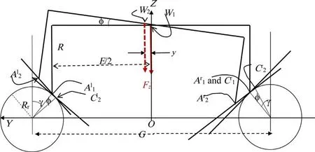
Fig. 1. Semi-simplified wheelset geometry of rigid rolling contact on curved rails ( G = E + 2 γ·R r ).
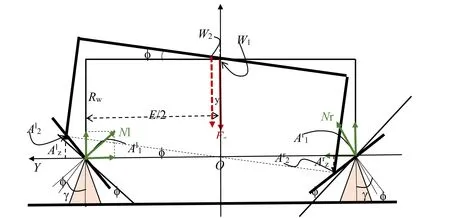
Fig. 2. Simplified wheelset geometry of rigid rolling contact on pointed rails ( G = E ).
Dynamical Equations of an unsuspended wheelset with zero frictionμ= 0.
Figure 1 shows the main geometry of a wheelset of which conical wheel tread profiles are perfect straight lines of constantγconicity (angle of the line slope in the wheelset reference). It has only 4 independent DoF because zero friction is set so that its forward velocityVxas well as the pitch velocities are not part to the problem.
Proper dynamical equations for Fig. 1 case are complicated if the rails radius is large because the localization of contacts depends on the roll angle. To simplify the problem we will focus on Fig. 2 when the rails are pointed with very small radii. Further tests using usual rails will show that Fig. 2 approximations stay within the wanted 1% accuracy.
A simplified geometry of this wheelset on pointed rails is presented on Fig. 2 and will be used below. For practical tests of commercial codes a specific rail profile with a 8 mm radius is provided in a supplementary Table, “8mm_radius_rail.txt” (rail profile on Fig. 12 ) in order to avoid the search of contact points localization on the rails.
In order to further simplify the case, both rails are represented in Fig. 2 as punctual fixed solids of which profiles are circles of neglectable radius, so that contact points are well located and normal forces directions are always normal to wheel tread profiles.The contact elasticity is set independently of the rail shape. The direct frameYOZhasOZpointing up andOYto the left. The positive roll angle is clockwise.
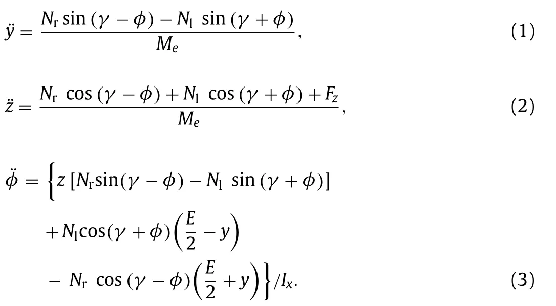
NewtonEquations
Since there is no friction, the sole forces acting on the wheelset are the vertical negative loadFzand positive left and right normal forces,Nl andNr . The three Newton equations are:
Eulerequationsandyawoscillations
Since there is no creepage forces, rotational moments would be due only to gyroscopic moments, and, at low forward speed and pitch velocity, it would be so small that we could ignore it and notably ignore the yaw oscillations also because they are not influencing the other DoFs. However, it will remain to verify this assumption by programming and solving numerically proper gyroscopic equations [10] that will act on roll,φand yawψ:
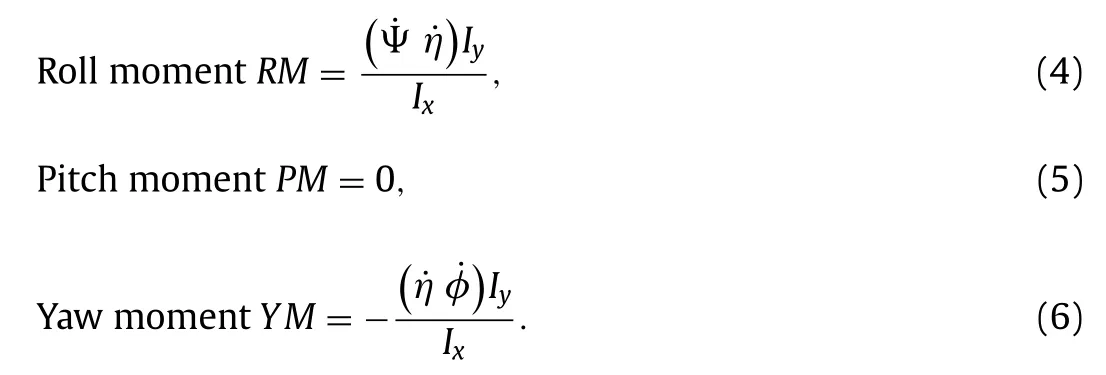
Note that, in programming the yaw moment, we have added small additional moments coming from the longitudinal displacements of the contact points linked to the yaw angle (see details in the Appendix Fortran code).
Assuming a periodic sinusoidal solution of angular frequencyω:
By assuming a sinusoidal solution with same oscillation frequencyωfor all DoFs, we derive direct equations between second derivatives and DoFs:
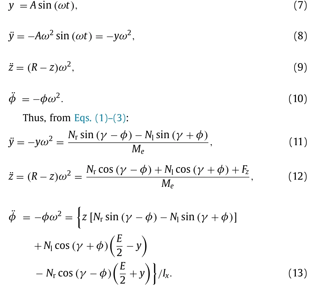
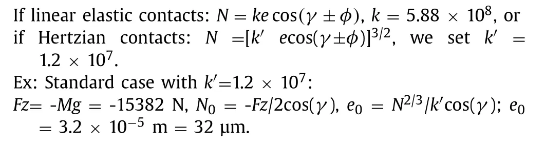
We will begin by calculating a numerical solution using elastic contacts allowing some small penetration,e, between wheels and rails, fromewe calculate the normal forces,N, using contact stiffnesses, Hertz’s or linear, and by assuminge= 0 we will calculate an analytical solution for the rigid case.
Contact stiffness:
Signsconventions
We set positive vertical penetration:e>0, and positive normal forces:N>0. Negativeemeans no wheel-rail contact, henceN= 0.
Left sideNlcalculation:
Knowing the wheelset situation [y,z,φ], we calculate the vertical penetrationeto determine the normal forceNlusing Hertzian stiffness.
The pointAl2 : [Aly,Alz] belongs to the left wheel tread. Wheny= 0, symmetric lowest situation,Alis on top of the pointed rail.We start from the wheelset center of gravityW2= [y,z]:
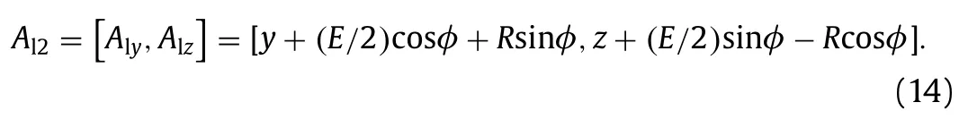
Then we recalculateAlzstarting from the contact point with -elvertical penetration, by equalizing both ways we get Eq. (16) :
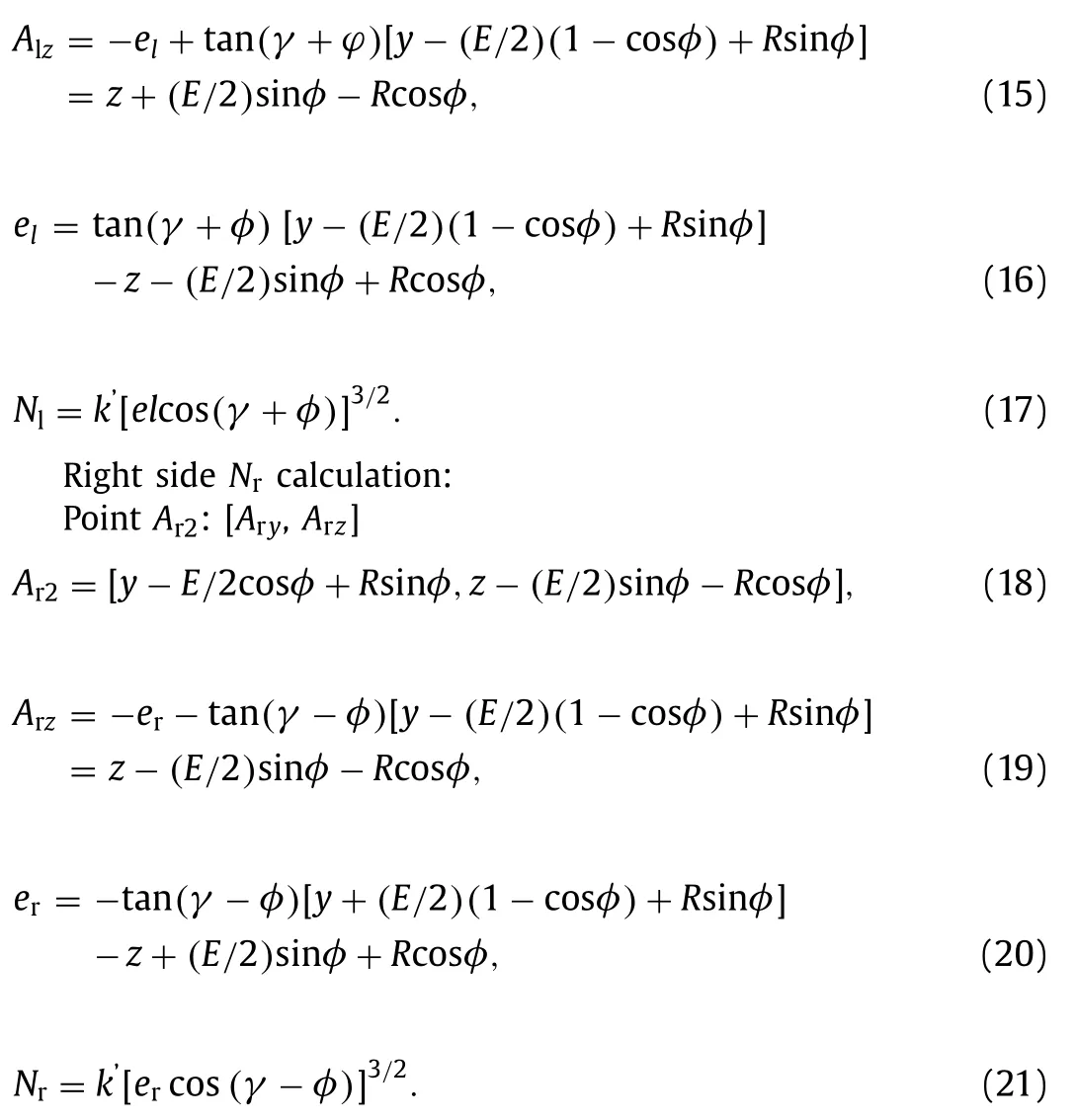
Rigidcontact
By settinger =el = 0 in Eqs. (16) and (20) , we get 2 new equations.
The last needed equation is given because the negative vertical loadFzmust be equilibrated by both normal loads:

“Pascal’s Formula”: Solvingω2from first order 6 equations (unknowns:y,z,φ,Nl,Nr,ω2).
When written at first order we will index equations with an upper prime, ex: Eq. (1 ′ ) or a double prime Eq. (1 ′′ ) for a most severe approximation.
Why not taking rotations into account for the new Formula?
By adding Euler equations we would have to write first derivatives introducing cos(ωt)so that Eq. (3) , even knowing constant the pitch velocity, ˙η=Vx/R, would loose its linearity inφand would complexify any attempt at analytical calculation ofω2:
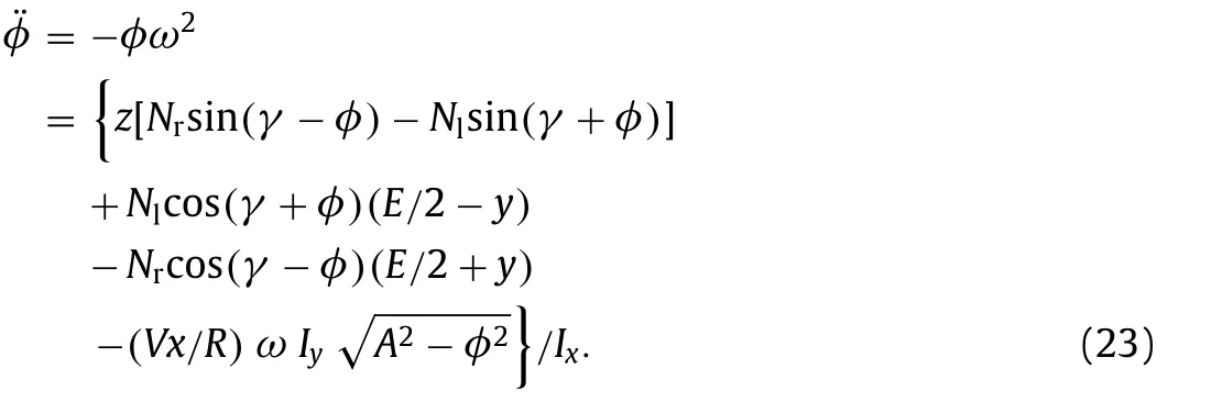
For this reason, we will try this calculation without Euler equations and no yaw degree of freedom and, later in this note, by solving numerically the full system, we will demonstrate that the amount of implied approximations is negligible for our formula validity.
Developingfirstorderequations
Thus, with 3 DoFs, 2 normal forces and the frequency unknowns, we have 6 equations and 6 unknows to solve the system and we should be able to calculateω2. But, because of having trigonometric functions in the equations, there would be no simple analytical solution. However, sinceγandφare small, we could try it at first order (sin(a) =aand cos (a) = 1) and settingel=er = 0 for a rigid contact.
Thus we linearize the 6 non-linear equations: Eqs. (1 )–(3) , (5) ,(7) and (9) in order to solve the system analytically. We are left to try first order approximations assuming that the conicityγis small (preferably 1/40) and that the roll,φ, can be set as small as necessary by minimizing initial conditions. Thus we rewrite equations at first order; sinceφ≪γ, we also eliminate some quadratic expressions: (φ2= 0), butγ φ/ = 0 :
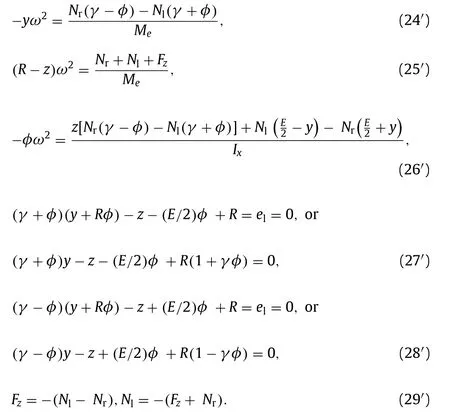
Figure 2 shows thatφ= (Alz-Arz)/E, thus we get Eq. (30), first order relationship betweenyandφ, by using Eqs. (15) and (19) at first order:

By using Eqs. (25) and (29), we come to(R-z)ω2= 0 . But,sinceω2= 0 would mean that there is no possibility of oscillations,then we must keepz=Ras a first order solution:
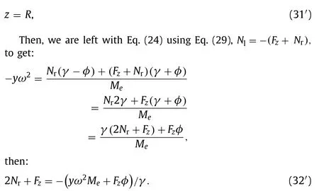
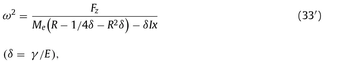
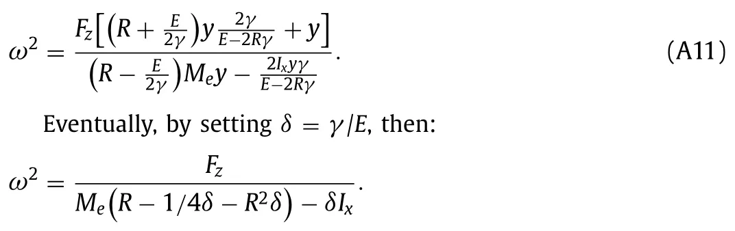
Using Eqs. (26), (29) and (32), we can solve the remaining set of equations to get Pascal’s formula (The detail of calculations is given in Appendix A ):
“Pascal’s formula” (μ= 0 )
Pascal’s formula assumptions:
1 Zero wheel-rail friction:μ= 0,
2 First order formulation of differential equations (conicityγand roll angleφare small),
3 Harmonic oscillations: ¨y= -ω2y,
4 Rigid contacts: large contact stiffnessk,k→ ∞ ,
5 No gyroscopic moments,.η= 0 .
To get a rough idea of main factors, sinceγis small, then Eq.(33) can be reduced with some reasonable approximation to:

And, with gravityg= 9.81 m/s2, we come toω2≈39.2(γ/E)which shows that the conicity and the gage are the main factors determining the wheelset-pendulum frequency.
Pascal’s simple formula
Standard case data:
We define a standard case which would fit usual wheelsets average dimensionsγ= 1/40, gageE= 1.515 m, wheel radiusR= 0.457 m, Wheelset massM= 1568 kg, inertiaIx=Iz= 656 kg ·m2,Iy= 166 kg ·m2, wheelset loadFz=Mg.
“Rigid-Hertzian” contacts:N= [k′ecos(γ±φ)]3/2, for rigid case we setk′ = 6 × 10⁹.
Ex: Standard CaseFz= -Mg= -15382 N,N0 = -Fz/ 2cos(γ).
Rigid case penetration:e0 =N2/3/k′ cos(γ) = 1.03 × 10⁻⁷ m = 0.1 μm.
“Pascal’s Formula” accuracy (limitation due to first order):
Numerical solver, stiffsolution, (in Table 2):ω2= 0.66251221 (rad/s)2.
Using Pascal’s formula from Eq. (33):ω2= 0.66719489 (rad/s)2,relative deviation: + 0.71%.
Numerical proper solver for very stiff elastic contacts:
We will integrate Eqs. (1 )–(3) with respect to time by using a specific numerical code (Supplementary ‘ZEROFRIC.for’) which develops Eqs. (16) , (17) , (20) and (21) to calculate step by step normal forces. The corresponding accelerations are integrated by a Taylor development using a very small time step necessary because of the large contact stiffness, see Ref. [8] . All parameters are double precision. The corresponding Fortran code is displayed with the input data file in (Supplementary ‘ZEROFRIC.for’).
Forward speed and pitch velocity = 0 to cancel gyroscopic moments.
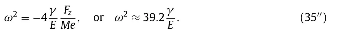
Table 1 shows the calculated oscillation frequencies of this wheelset whilst variating gravity (wheelset load) and contact stiffness, together with deviations of the “Pascal’s Formula”. Table 2 shows the same for rigid contact cases variating wheelset geometry.
Figures 3–7 show displacements and normal forces in the case of usual gravity (9.81 m/s2). The application code ZEROFRIC.exe is stable for contact stiffnesses at least up to 10 0 0 times higher than usual Hertz stiffness, see Ref. [8] . This case is said “stiff” or rigid contact because wheel/rail penetration is calculated lower than 0.1 μm and it can be very close to the proper rigid contact solution.
These results show that the proposed formula provides a reliableω2frequency, within 1% accuracy, for wheelset practical di-mensions. Simulations demonstrate that wheelset oscillations are harmonic (see Fig. 8 ).
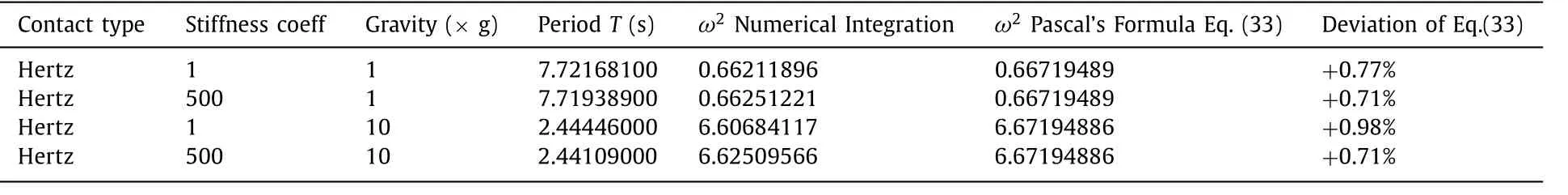
Table 1 Calculated wheelset frequency as function of contact stiffness and gravity, V x = 0 (Coeff. 1 = Hertz stiffness for loaded nonconformal wheels on usual rails).
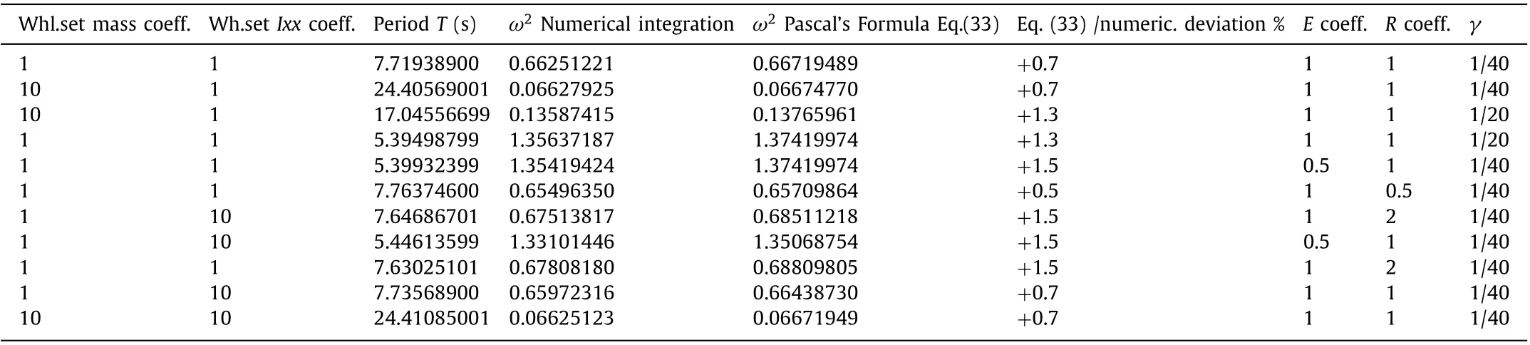
Table 2 Calculated wheelset frequency varying g, E, R, M, Ixx , with Fz constant, V x = 0 (Hertz contact stiffness × 500, constant vertical load: Fz = 1568 × 9.81 N; 1 = standard case data).
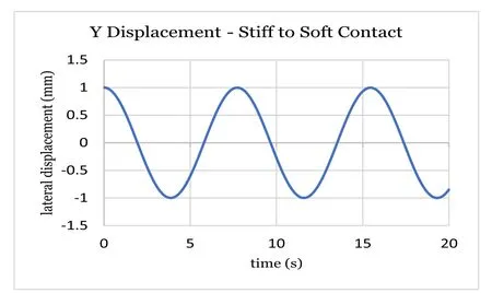
Fig. 3. Lateral Y displacement.
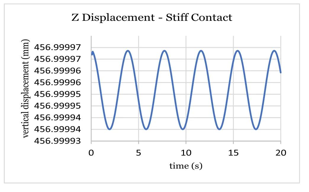
Fig. 4. Vertical Z displacement (stiff).
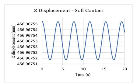
Fig. 5. Vertical Z displacement (soft).
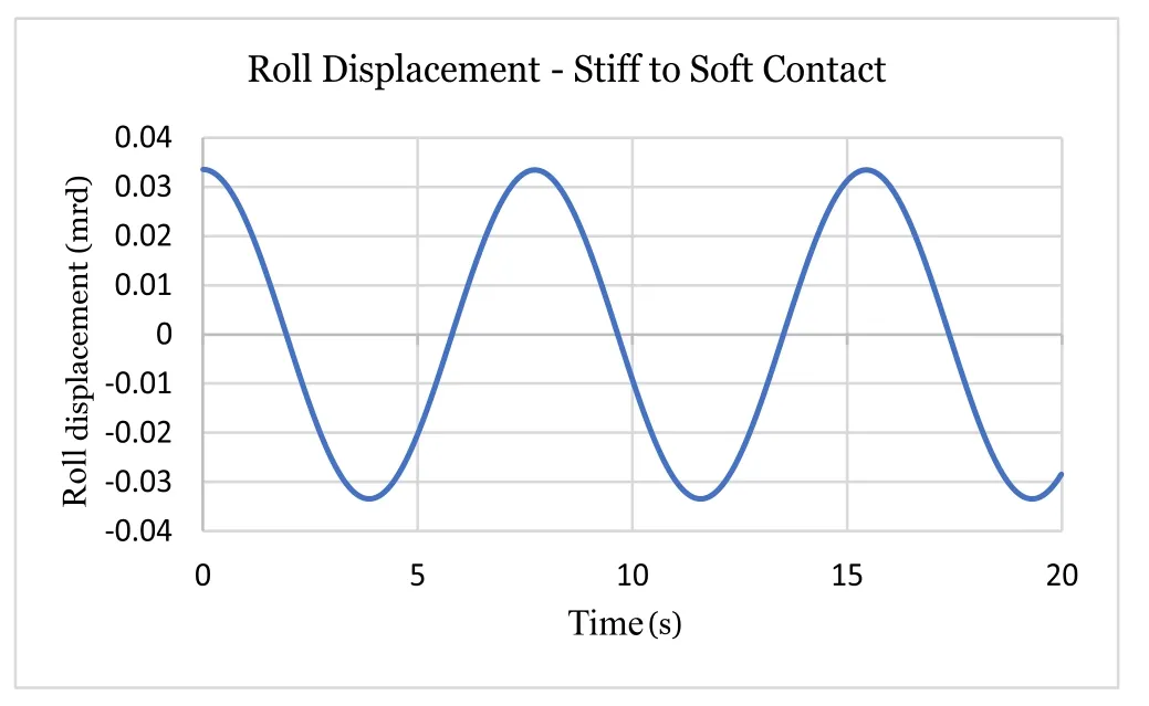
Fig. 6. Roll φ displacement.
Pitch velocity / = 0, rotational equations and yaw DoF.
Up to now we have assumed that, since there is no creepage forces, rotational moments, rotation velocity and thus yaw angle would be so small that we could ignore it and notably ignore the yaw oscillations because it does not influence the other DoFs. It now remains to verify this assumption by programming proper gyroscopic equations that will act on roll,φ, and yaw,ψ,φfrom Eqs. (4)–(6) , and by setting initial forward and pitch non zero velocities,Vxand ˙η; the pitch velocity, ˙η, is set according to:


Table 3 Calculated wheelset frequency as function of rotation velocity (gyroscopic mom.) (Hertz contact stiffness ×500, standard case data).
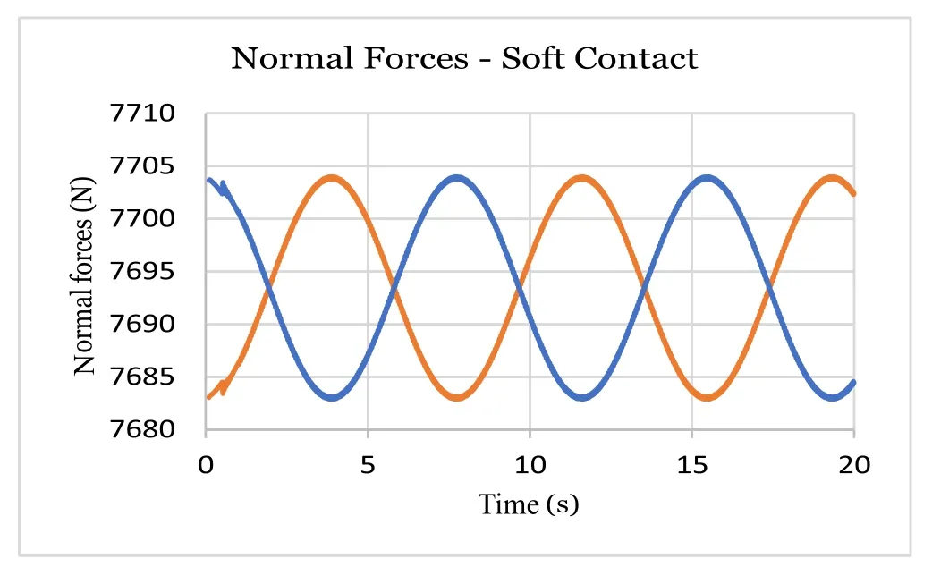
Fig. 7. Normal forces.
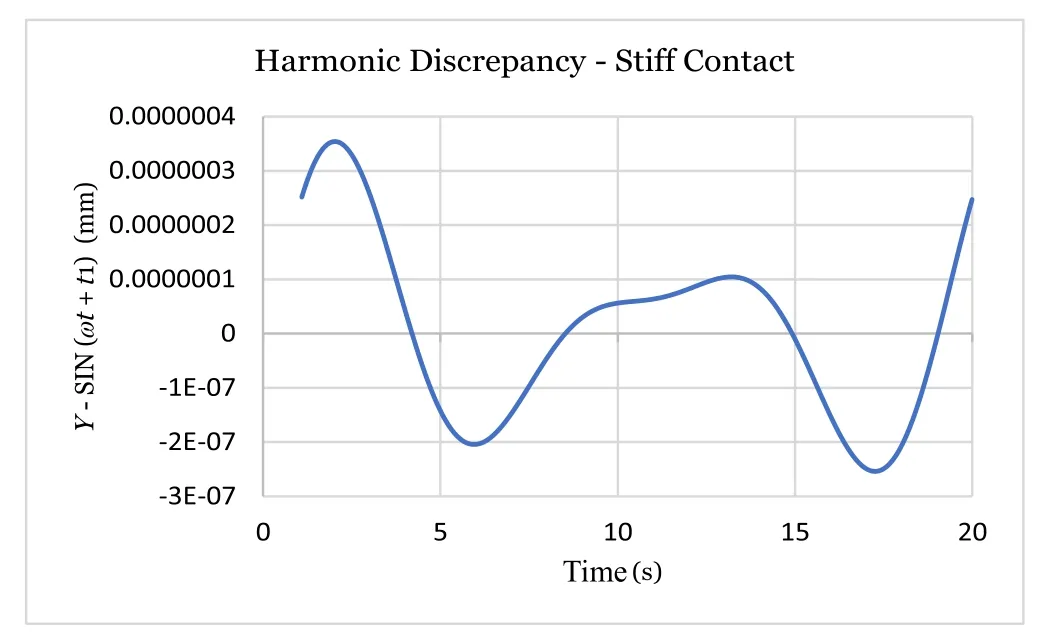
Fig. 8. Y deviation from a sine < 3 × 10⁻⁵ %.
Note that, in the yaw moment, we have added small additional moments coming from the longitudinal displacements of the contact points linked to the yaw angle (see details in the Fortran code).
Table 3 shows the results of the numerical solver ‘ZEROFRIC.exe’(code in Supplementary ‘ZEROFRIC.for’). Fig. 9 shows the yaw oscillation and Fig. 10 shows the phases of yaw moments.
With 1mm lateral displacement and ˙η= 219 rad/s (Vx= 100 m/s),the yaw angle is smaller than 3 mrad ( Fig. 9 ), and the deviation ofω2is only 0.3% from the caseVx= 0. AtVx= 10 m/s ( ˙η= 21.9 rad/s),the 0.0033% deviation can be forgotten.
On Fig. 10 the blue line shows the gyroscopic yaw moment at 1.5 mN ·m and the orange line shows the ( × 100) stabilizing moment generated by the longitudinal displacement of contact points at 7 × 10⁻⁶N ·m, 20 0 0 times smaller than the gyroscopic.
Note: Since there is no damping in the system, if the average yaw velocity is not initially zero, then nothing will correct it and the yaw displacement would shift continuously. Thus it is necessary to initially damp the system in order to get a clean oscillation when all damping stops (here att= 12 s); this damping moment is presented by the green line on Fig. 10 .
Standardcasesolutions
γ= 1/40,Me= 1568 kg,Ix=Iz= 656 kg ·m2,Iy= 168 kg ·m2,E= 1.515 m,R= 0.457 m,Vx= 6.7 m/s (15 mph).
Numerical solver target solution:ω2= 0.66252233 (rad/s)2.
Pascal’s Formula Eq. (33):ω2= 0.66719489 (rad/s)2( + 0.7%).
As commercial codes use digitalized files to characterize wheels and rails profiles, although any constant conicity profiles could do,two verified clean profiles are given as attached table files. The rail profile (Supplementary Table ‘8mm_radius_rail.txt’) was specifically made to have a small radius at contact points ( Fig. 12 ), occurring very near the rail zero abscissa, and thus providing a precise contact localization and thus accurate distanceE. The wheel profile ( Fig. 11 ), (Supplementary Table ‘1_40 verified Wheel.txt’), has enough points so that its 1/40 slope, about the zero abscissa where the contact points should be set, and the slope derivatives are quite constant and continuous. Although any usual profiles could work for this test (see below), it is better to use our profiles because,due to the lack of any damping, using approximative profiles, it would suffice of a light lateral wheelset shift to result in different right and left conicities, hence the pendulum oscillation would be perturbated and its frequency measurement would be approximative.
Testing online calculation of railway elastic contacts (OCREC)code [ 11 , 12 ].
For this test, a wheel profile with a constant verified conicity tread is necessary. Such a profile with 1/40 conicity is attached in the supplementary file ‘1_40 verified Wheel.txt’ (it is a copy of the SNCF TGV 1/40 profile); this wheel profile hasy= 0 andz= 0 at the middle of the tread. The contact point should be chosen about the middle of the tread, which is at 80mm from the back of this wheel.To this effect, we adjust the input parameter back-to-back distance of the wheels: to simulate our standard case (E= 1515 mm), we have to set the back-to-back at 1355 mm (1515-2 × 80). The top of this rail is at 40 mm from the gage point, thus we set the track gage at 1.435 m (1.515-0.080). Note from Eq. (33) that this parameter E is sensitive and must be set accurately.
For this benchmark a specific rail profile has been designed( Fig. 12 ) with a small top radius (8 mm) in order to get easily a precise localization of the contact point which can be taken at the rail top.
This rail profile, in Supplementary Table “benchmark_rail.txt”,hasy= 0 andz= 0 at the rail top.
Note again that this parameter E is sensitive and must be known accurately so that contact points distanceEshould be well known.
Since oscillations figures of OCREC simulations are the same as Figs. (3)–(8) , only the lateral displacement and the yaw angle due to gyroscopic moments are presented here in Figs. 13 and 14 .
Thus, using OCREC code we get a periodt= 7.683 ±0.01 s and an oscillation frequencyω2= (2π/t)2= 0.6687 (rad/s)2, close to the numerical exact target solution of our test,ω2= 0.6625 (rad/s)2,ω2= 0.6687 (rad/s)2(-0.02%<ε<+ 0.5%), the relative deviationεis related to “Pascal’s Formula”, and if the deviationεwould be related to the numerical ‘target value’, we would getε=+ 0.93%.
Target value = numerical exact solution:ω2= 0.6625 (rad/s)2,
‘Pascal’s formula:ω2= 0.6672 (rad/s)2,
Using OCREC code:ω2= 0.6687 (rad/s)2.
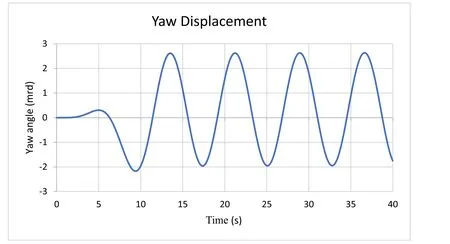
Fig. 9. Yaw angle ( ˙ η = 219 rad/s).
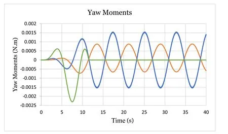
Fig. 10. Yaw moments. Blue: gyroscopic, green: init.damping ( × 100), orange: due to longi.cont.displ.( × 100).
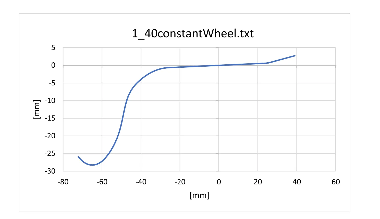
Fig. 11. Wheel profile (‘1_40 verified Wheel.txt’).
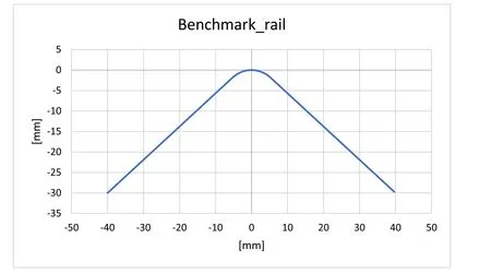
Fig. 12. Rail profile (‘8mm_radius_rail.txt’).
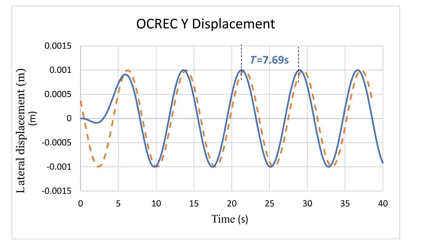
Fig. 13. OCREC lateral displacement standard case t = 7.683 s, ω 2 = 0.6687. Dotted orange line: target case.
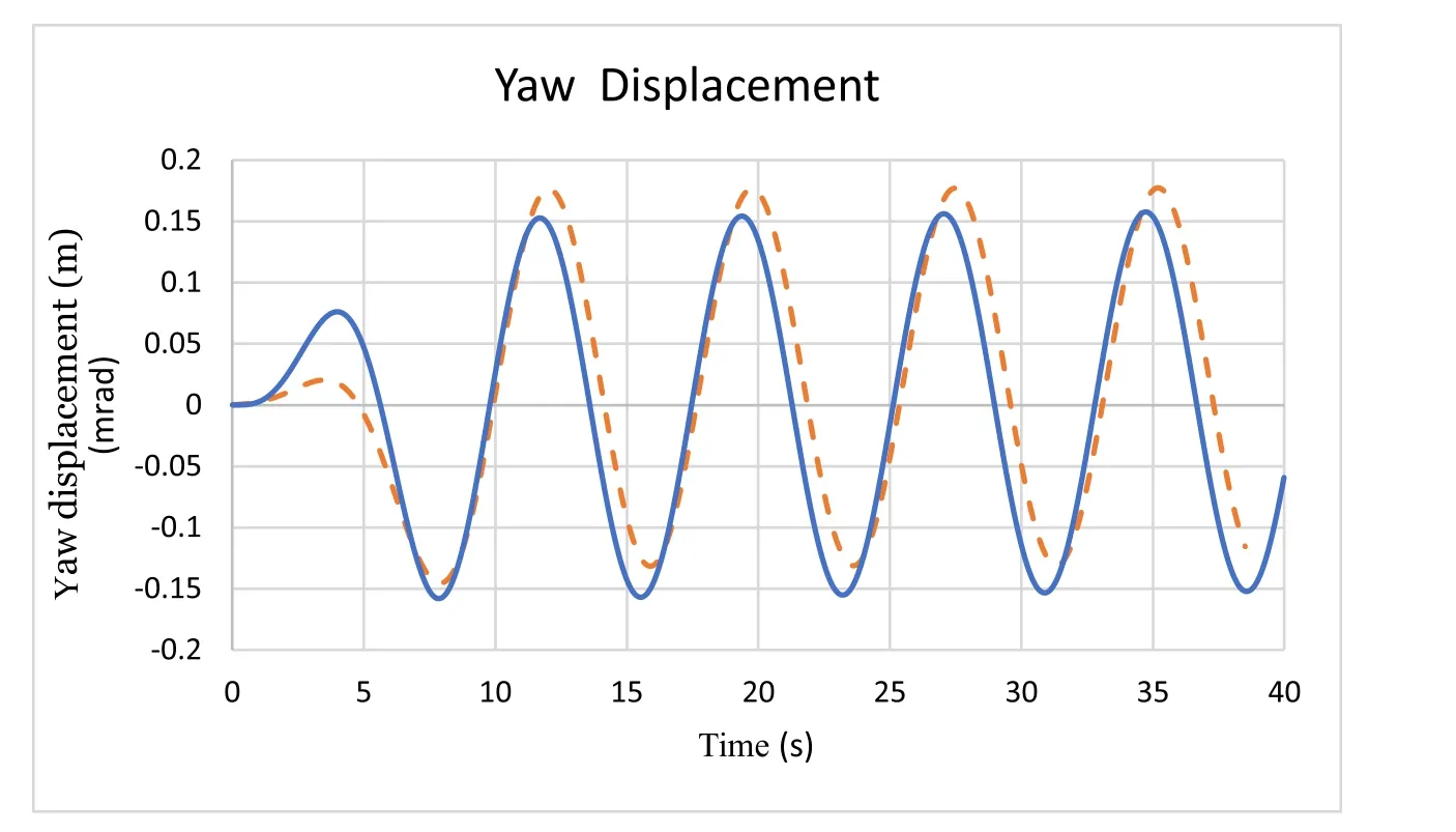
Fig. 14. OCREC yaw displacement standard case, V x = 6.7 m/s, ˙ η= 14.66 rad/s Dotted orange line: target case OCREC solution for the Standard case.
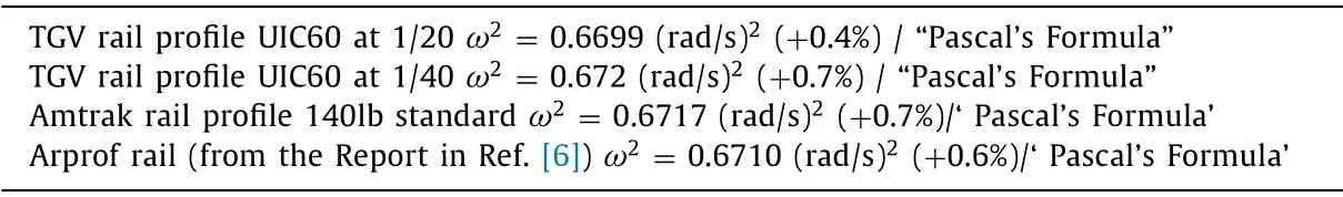
Table 4 Solutions of OCREC code using usual rails.
Thus, OCREC code calculatesω2within 1% off Pascal’s Formula,meaning that there should be no doubt about its coding. By adjusting the gage so as to get the same distanceEat 1.515 m, we used different rails which have different top radii and we also got,in Table 4 , oscillation frequencies within 1% from Pascal’s Formula.
While using usual friction coefficients (0.1<μ<0.5) and conicities (1/40<γ <1/20), unsuspended running wheelsets are hunting,the wheel-rail slippage is so small that the natural hunting frequency could be calculated precisely by Klingel (1883) in an analytical famous formula, Klingel’s Formula [1] . When there is no friction, there is wheel-rail slippage, Klingel’s formula does not apply and we have calculated a new formula, “Pascal’s Formula”, Eq.(33), which gives a close approximation of the square of the angular wheelset oscillation frequency for the no-friction cases.
We have demonstrated, for usual wheelsets dimensions, that,in spite of the first order and zero interpenetration formula limitations, the accuracy of this formula is in the range of 1% and thus allows to use it as a target to verify the proper formulation of commercial codes or to help developing new codes either using rigid or elastic contact formulations.
Since the formula showsω2as a dependent function of the distanceEbetween contact points, it is necessary to evaluate preciselyEwhen testing a code with digitalized profiles. Similarly, the wheels conicity must be known and be independent from small displacements, which is related to the wheels tread profiles to be straight. To avoid possible issues, avoiding to pre-measure the localization of contact points on the rails, we provide a file of a rail profile with a small top radius (8 mm) such that the top, at abscissa zero, can be taken as the contact point localization (Supplementary Table ‘8mm_radius_rail.txt’).
To avoid gyroscopic and yaw angle unexpected drifts, we recommend to make the tests of the codes at low rotation velocity<10 m/s.
If high speeds and high wheelsets rotation velocities would be wanted, it would be appropriate to verify that the yaw angle does not drift toward unrealistic large values. Initial conditions could be activated by some small (<1 mm) lateral displacement of the track,preferably in the form of a cosine lateral bump of same wavelength as the predicted oscillation at the given speed in order not to excite undesirable high frequencies. Since the frequency is measured with no damping at all, any excited frequencies would not stop and could perturbate the main pendulum harmonic oscillation.
We have calculated the angular frequency of an unsuspended wheelset for cases with zero wheel-rail friction and we provide a first order analytical formula for that calculation. In spite of the first order and zero interpenetration formula limitation, we have evaluated the frequency calculated by Pascal’s formula to be within 1% off the full integrations without approximations in cases of usual wheelsets dimensions and usual wheels conicity.
Thus we believe that this study will help to improve coding dynamical MBS codes by providing a new simple and accurate formula as a target to their numerical results.
Declaration of Competing Interest
I have no conflict of interest with this publication.
Acknowledgements
The idea that dynamical simulations of isolated wheelsets with zero wheel-rail friction is worth studying comes from Dr. J.R. Sany.There has been no external funding for this research.
Appendix A
Developments: How to get “Pascal’s Formula”, Eq. (33), from Eqs. (26), (29) and (32):
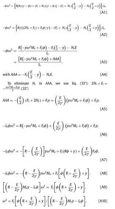
Eventually, we eliminateφusing Eq. (30’),φ= 2yγ/(E-2Rγ):
 Theoretical & Applied Mechanics Letters2022年3期
- Theoretical & Applied Mechanics Letters的其它文章
- Importance of induced magnetic field and exponential heat source on convective flow of Casson fluid in a micro-channel via AGM
- Optimal thermal design of anisotropic plates with arbitrary cutouts using genetic algorithm
- Optimal patching locations and orientations for maximum energy harvesting efficiency of ultrathin flexible piezoelectric devices mounted on heart surface
- Similarity solutions of Prandtl mixing length modelled two dimensional turbulent boundary layer equations
- Numerical simulation of droplet coalescence based on the SPH method
- Thermal energy storage inside the chamber with a brick wall using the phase change process of paraffinic materials: A numerical simulation