
Spatially modulated scene illumination for intensity-compensated two-dimensional array photon-counting LiDAR imaging
2022-09-24 07:59JiahengXie谢佳衡ZijingZhang张子静MingweiHuang黄明维JiahuanLi李家欢FanJia贾凡andYuanZhao赵远
Chinese Physics B 2022年9期
关键词:李家
Jiaheng Xie(谢佳衡), Zijing Zhang(张子静), Mingwei Huang(黄明维),Jiahuan Li(李家欢), Fan Jia(贾凡), and Yuan Zhao(赵远)
School of Physics,Harbin Institute of Technology,Harbin 150001,China
Keywords: avalanche photodiode camera,photon counting,three-dimensional imaging,array modulation PACS:07.05.Pj,42.30.-d,42.68.Wt DOI:10.1088/1674-1056/ac5e96
1. Introduction
Photon-counting LiDAR using picosecond laser and Geiger-mode avalanche photodiode (GM-APD), combined with time-correlated single photon counting technology(TCSPC),[1,2]can realize three-dimensional imaging in longdistance[3-6]and low illumination power[7,8]environments.Current photon-counting LiDAR systems can be categorized into three types. The first type of system is composed of a single-pixel GM-APD combined with a 2-axis scanning device.[4,9-11]The scanning device is mainly a mechanical rotating platform[12]or a galvo scanner.[13]The second type of system is composed of a 1D GM-APD array combined with a 1-axis scanning device.[14]The third type of system uses a 2D GM-APD array with or without a scanning device.[15-18]The lateral imaging resolution and acquisition speed of the last type of systems can be beneficial by the considerable number of detectors. With the development of all-digital complementary metal-oxide semiconductor(CMOS)technology for GMAPD,[19,20]the 2D GM-APD arrays[21,22]have become accessible to photon-counting LiDAR systems. The increase in the number of detectors demonstrate the superiority of the 2D array photon-counting LiDAR in practical applications.
Intensity and depth are the two most important pieces of information in 3D imaging. Two-dimensional array photoncounting LiDAR requires flood illumination of the scene. The non-uniform intensity profile of the illumination beam introduces additional errors in the intensity image, which causes significant challenges to the subsequent image denoising process and target recognition. The limitation of the current array manufacturing is spatial non-uniformity. For example,the 2D GM-APD arrays have neither the same quantum efficiency nor the same noise characteristics.[23]This non-uniformity leads to fluctuations in the number of photoelectrons that are generated by the received photons and consequently degrades the image quality. Two-dimensional array photon-counting Li-DAR needs to solve these problems in practical applications.
In view of the image quality deterioration caused by the non-uniform intensity profile of the illumination beam and non-uniform quantum efficiency of the detectors in the 2D array, this study proposes a novel 2D array photon-counting LiDAR system that uses a spatial light modulator in the illumination channel to control the spatial intensity of the illuminating beam. By controlling the spatial intensity to compensate for both the non-uniform intensity profile of the illumination beam and the variation in the quantum efficiency of the detectors in the 2D array, an accurate intensity image can be obtained. Simulations and experimental results verify the effectiveness of the proposed method. Specifically, compared with the unmodulated method, the standard deviation of the intensity image of the proposed method is reduced from 0.109 to 0.089 for a whiteboard target,with an average signal photon number of 0.006 per pixel.
2. Photon counting LiDAR with spatially modulated illumination
2.1. System
Figure 1 shows a schematic diagram of the photoncounting LiDAR system with spatially modulated illumination. The transmitter is composed of a laser, three lenses, a phase modulation mode spatial light modulator (SLM), and an analyzer. The emitted laser is firstly expanded by the lens 1 and lens 2, and then incident on the spatial light modulator. An analyzer and a spatial light modulator constitute a transmission-power regulator. Different gray values of the spatial light modulator correspond to different optical transmittances. In this system,a gray modulation matrix is loaded onto the spatial light modulator to realize the lateral pixel-level modulation of the illumination beam intensity.Lens 3 projects the spatially modulated beam to illuminate the scene. The receiving part of the system consists of an imaging lens and a single-photon avalanche diode (SPAD) camera. The field of view (FOV) of the camera coincides with the spatially modulated illumination beam. A signal generator provides a synchronization signal for the laser and SPAD camera.
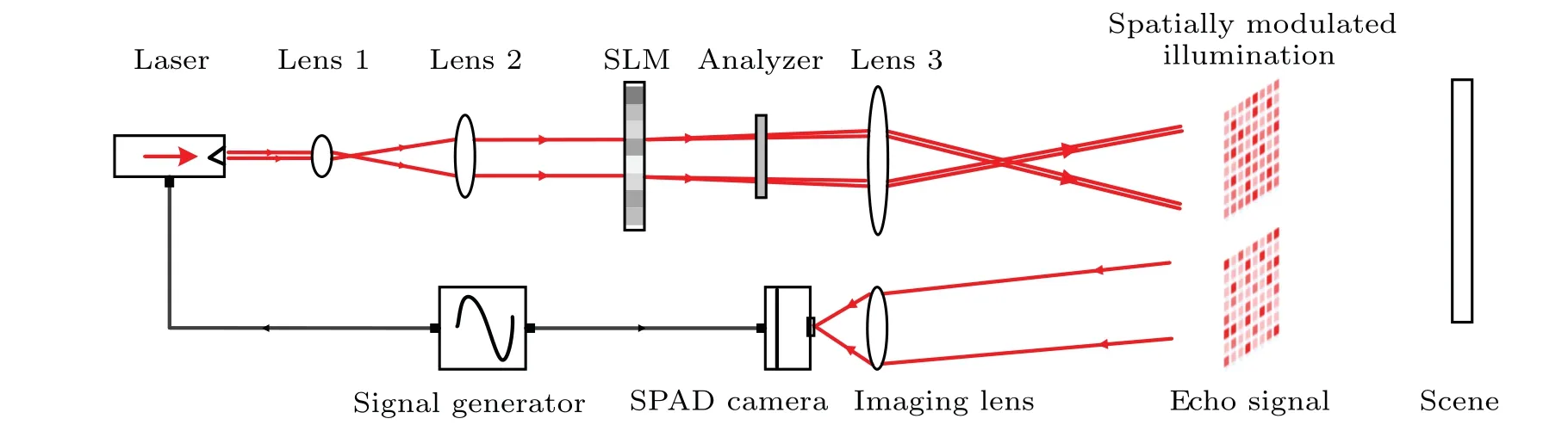
Fig.1. Schematic diagram of the photon counting LiDAR system with spatially modulated illumination.
2.2. Model and method
Semiconductor lasers have multiple advantages, such as small size, low power consumption and low cost. Because a laser diode (LD) is used in our system, the theoretical analysis and simulations are all based on the laser diode. Laser diodes have different waveguide structures in two directions,that is, perpendicular and parallel to the heterojunction. An asymmetric Gaussian function was used to describe the spatial intensity distribution of the laser beams emitted by the LD.[24]The intensity distribution field can be expressed as
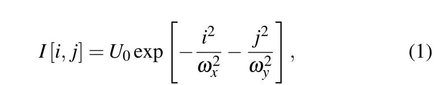
whereU0is the normalized quantity of the beam.ωxandωyare the waist radii in thexandydirections,respectively.iandjare the discrete variable forms ofxandy. Figure 2 shows an example of the simulated spatial intensity distribution of the laser beam. The waist radii of this example areωx=0.08 m andωy=0.04 m,respectively.
Suppose that the temporal profile of the laser pulse ish[k].kis the discrete sampled version of timet. The reflectance and distance of the target areρ[i,j]andR[i,j],respectively. Each pixel of the SPAD camera has a different dark count noised[i,j] and quantum efficiencyη[i,j]. The aperture area of the imaging lens isAR.N0is the total number of photons of the beam. Then,the number of photons received by the SPAD camera can be expressed as

After spatial modulation, the average number of signal photons at each pixel is expected to be the same and is expressed as
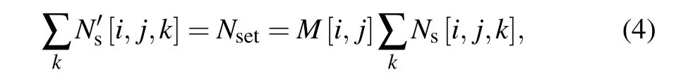
whereNsetis the preset average number of signal photons at each pixel. Therefore,the modulation matrix of the SLM can be calculated as
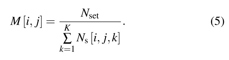
Thus far,we have obtained the modulation matrix of the SLM using a whiteboard target with uniform reflectance. For other scenes and targets,a more accurate imaging result can be obtained by setting the SLM modulation matrix toM[i,j].

Fig.2.Spatial intensity distribution of laser diode.(a)Two-dimensional view. (b)Three-dimensional view.
The probability of photon detection in a histogram bin can be modeled as a Poisson distribution.[14]Aftermpulses illumination,the captured photon count histogram at the pixel[i,j]within thekth time bin is distributed as where 2D matrixYis the number of signal photons of each pixel captured in the photon count histogramy. Twodimensional matrixXis the estimate of the correct intensity image after denoising. Total variation penalty term TV(·)enforces the smoothness in the intensity solution. As one of the most effective tools for image denoising, the total variation method can perfectly preserve the edge of an object after denoising, which has attracted wide attention.[25,26]εis a positive scalar parameter that determines the degree of smoothness. Because we chose complex natural scenes as imaging targets, the sparsity of intensity images, such as thel1norm penalty andl2norm penalty were not used here. When working in high-noise scenarios (such as daytime environments),our system can still improve the image quality limited by the non-uniformities of the illumination beam and detector array.The modulation matrixM(i,j) can be calculated in a lownoise environment before the measurements with high ambient noise. Efficient denoising methods, such as global gating[4]and the unmixing method[27]can be used to eliminate the detected background noise.
3. Simulation analysis
Based on the theoretical model in Section 2, we carried out numerical simulations to evaluate the performance of the conventional method and the proposed method with different illumination and detector conditions.In addition,a link budget analysis was included to indicate the scenarios which would benefit most from the proposed method. The simulation parameters were selected as consistent with the laboratorial system parameters as far as possible. In the simulations,a total of 20000 laser pulses were accumulated to generate a temporal histogram. The lateral imaging resolution was 32×32 pixels.A laser diode was used for the floodlighting. The full width half maximum(FWHM)of the laser pulse was 400 ps,and its temporal profile was a Gaussian function. The FWHM of the total temporal impulse response was 700 ps. Each laser pulse sent out from the transmitting end had an average number of 9×10⁷photons. The time bin width of the photon counter was 55 ps, with a total of 1024 time bins. A planar target at the 518th time bin(corresponding to a distance of 4.27 m)was used for imaging. Its reflectivity was uniform (ρ=0.5)with a size of 32×32 pixels. The background noise and dark count noise wereb= 1.2×10⁻⁴andd= 9.8×10⁻⁹(corresponding to 100 Hz per pixel), respectively. The diameter of the receiving optical lens was 8.9 mm. In the simulations,the combination of the SLM and analyzer was considered to have perfect intensity modulation. The preset average number of signal photons per pixel in the proposed method wasNset= 0.006. The standard deviations of the intensity and depth images were used to quantitatively evaluate the performance of the two methods. The standard deviations of the intensity and depth images are calculated as
where ¯Iand ¯Rare the mean of the intensity and depth images of the measurements, respectively.I[i,j] andR[i,j] are the intensity and depth values at pixel [i,j], respectively.MandNare the total number of pixels along thex-andy-directions,respectively.
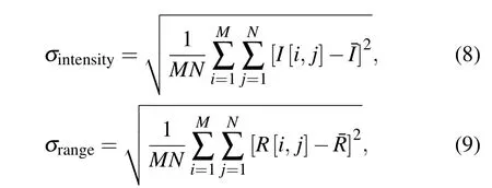
3.1. Standard deviation of the illumination beam intensity
In these simulations, we tested the performance of the conventional and proposed methods with different standard deviations of the illumination beam. The standard deviations of the illumination beam were set to be 3.5×10-4,3.7×10-4,3.9×10-4, ..., 13×10-4. Here, a different standard deviation was realized by changing the illumination beam waist radiiωxandωyin Eq. (1). The waist radii of the illumination beam wereωx=80 mm, 86 mm, 92 mm,..., 194 mm,andωy=ωx/2. The mean photon detection efficiency of the detector array was assumed to be 20%.
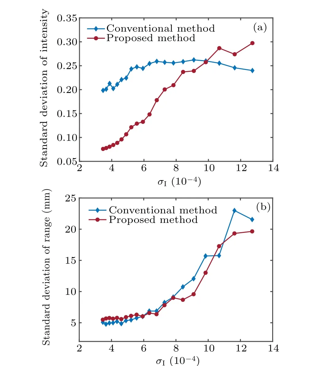
Fig.3.Simulation results of the conventional and proposed methods under different illumination conditions.(a)Standard deviation of intensity versus standard deviation of the illumination beam. (b)Standard deviation of the depth versus standard deviation of the illumination beam.
Figure 3(a)shows the curves of the standard deviation of the intensity image versus the standard deviation of the illumination beam. As the standard deviation of the system illumination beam increases from 3.5×10⁻⁴to 13×10-4, the standard deviation of the intensity with the conventional method increases from 0.20 to 0.24. The standard deviation of the intensity with the proposed method increases from 0.07 to 0.3. Figure 3(b) shows the curves of the standard deviation of the depth versus the standard deviation of the illumination beam. With an increase in the standard deviation of the illumination beam, the standard deviation of the depth with the conventional method increased from 5 mm to 22 mm,and the standard deviation of the depth with the proposed method increased from 5.5 mm to 20 mm.In the case of different illumination conditions, the proposed method effectively improves the uniformity within the range of 3.5×10⁻⁴to 10×10-4of the standard deviation of the illumination beam.
3.2. Standard deviation of quantum efficiency
In these simulations,we assessed the performance of the conventional and proposed methods with different standard deviations of the quantum efficiency of the detector. The quantum efficiency of the SPAD camera was non-uniform and obeyed the normal distributionη(i,j)~N(0.2,ση), whereση=0.005,0.01,...,0.1. Therefore,the standard deviations of the detectors’quantum efficiency were 0.005,0.01,...,0.1.The waist radii of the transmitted beam wereωx=182 mm andωy=91 mm. Figure 4(a)shows the curves of the standard deviation of intensity versus the standard deviation of quantum efficiency.
Fig.4.Simulation results of the conventional and proposed method with different detectors’quantum efficiency. (a)Intensity standard deviation versus standard deviation of quantum efficiency. (b) Depth standard deviation versus standard deviation of quantum efficiency.
It can be noted from the intensity results that using the proposed method, the standard deviation of the intensity decreases.As the non-uniformities in the detector array increase,the standard deviation of intensity of the proposed method increases from 0.08 to 0.16, while that of the conventional method decreases from 0.21 to 0.18. The proposed method effectively alleviates the degradation of the quality of the intensity image due to the non-uniform quantum efficiency of the detector array.Figure 4(b)shows the curves of the standard deviation of the depth versus the standard deviation of the quantum efficiency. For the depth results, both the proposed and conventional methods had a similar performance. The standard deviation of depth increases from 5.8 mm to 7.0 mm and 5.0 mm to 6.1 mm for the proposed and conventional methods,respectively.
3.3. Link budget analysis
Through a spatial light modulator, the proposed method alleviates the degradation of image quality due to the nonuniform illumination beam and non-uniform quantum efficiency of the detector array. For a photon-counting LiDAR,the non-uniformity of the illumination beam can be improved by expanding the Gaussian beam to be much larger than the field of view of the detector array. It is meaningful to compare the applicability of the beam-expansion method with that of the proposed method. In this simulation,we compared the performance of the proposed method,the conventional method without beam expansion, and the conventional method with double beam expansion at several distances. The quantum efficiency of the SPAD camera obeyed the normal distribution,η(i,j)~N(0.2,0.05). For the conventional method without beam expansion and the proposed method, the waist radii of the illumination beam wereωx=182 mm andωy=91 mm.For the conventional method with double beam expansion,the waist radii of the transmitted beam wereωx=364 mm andωy=182 mm. The distances of the planar target were 1 m,1.5 m, 1.9 m,..., 10 m (corresponding to the 121st, 179th,236th,..., 1212th time bins, respectively). The number of time bins of the photon counter was increased to 2048.
Figure 5(a) shows the curves of the mean number of received signal photons per pixel versus the object distance. In this case, the mean number of received signal photons per pixel using the proposed method was less than that of the conventional method without beam expansion. The mean number of received signal photons by using the conventional method with double beam expansion was less than that of the proposed method. Part of the energy was lost through beam expansion.Figure 5(b) shows the curves of the intensity standard deviation versus the object distance. The standard deviation of intensity of the conventional method with double beam expansion was lower than that of the conventional method without beam expansion, while the standard deviation of intensity of the proposed method was lower than that of the above two methods. The standard deviation of intensity was more improved using the beam expansion method than the unexpanded method. It improves the intensity image quality by sacrificing part of the energy. For practical applications,it is necessary to consider the balance between energy loss and the improvement of illumination uniformity. Compared with the conventional method with double beam expansion,the proposed method is more appropriate for imaging systems with non-uniform array detectors.
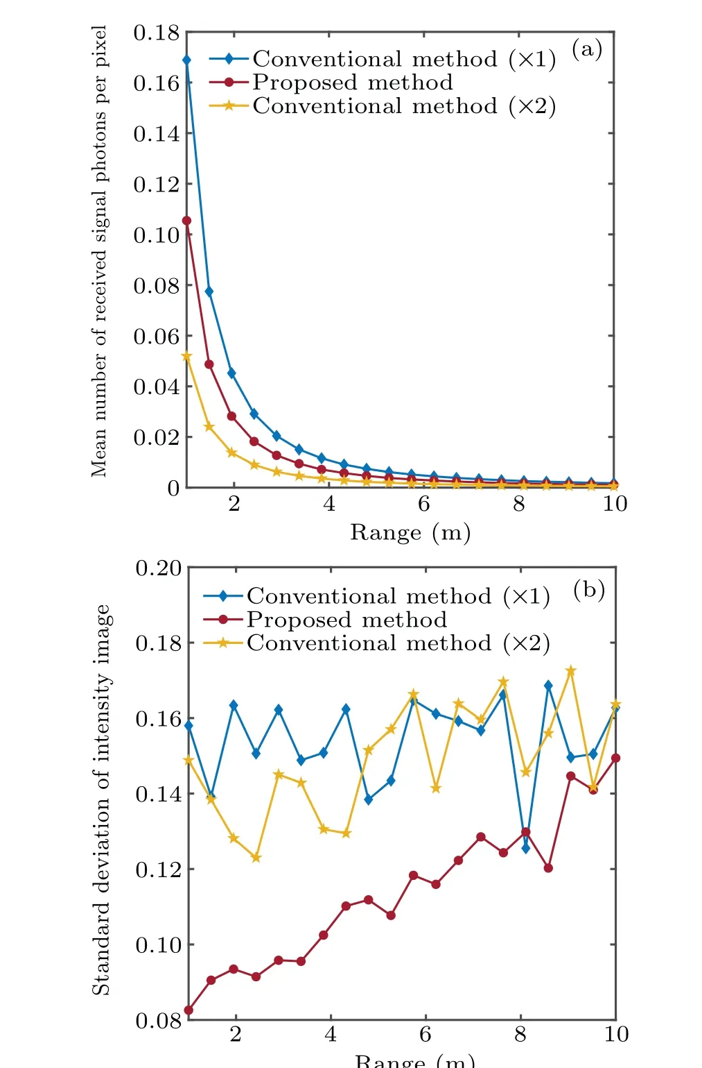
Fig.5. Simulation results of the conventional method without beam expansion,conventional method with double beam expansion and the proposed method at several object distances. (a)Mean number of received signal photons per pixel versus object distance. (b)Standard deviation of intensity versus object distance.
4. Experiment results
Figure 6 shows a built-up photon-counting LiDAR system with spatially modulated illumination. We experimented by using a 400 ps FWHM pulsed semiconductor laser (Pico-Quant LDH P635) with 635 nm peak wavelength, 4 mW average power when operated at a repetition rate of 10 MHz, a SPAD camera(Photon Force,PF32)with 32×32 pixels,mean quantum efficiency of 20%at a wavelength of 635 nm, and a built-in TCSPC module with 55 ps temporal resolution,1024 time bins and 100 Hz average dark counts. The FWHM of the total temporal impulse response was 700 ps. The SPAD camera used a lens (NAVITAR, ZOOM 7000) with an aperture of 8.9 mm and a focal length of 50 mm. A signal generator(Tektronix AFG3252)provided a 10 MHz square wave synchronization signal for the laser and the SPAD camera. A phase modulation mode SLM (Daheng optics, GCI-770202)combined with an analyzer was added to spatially program the illumination beam. The number of pixels in the SLM was 1920×1080. This is a transmission-type modulator. By controlling the gray value of a single pixel of the SLM, the polarization direction of the transmitted light is changed.[28]Then, it was combined with the analyzer to adjust the power of the emitted laser.Finally,the spatially modulated beam was projected by a lens to achieve programmed spatially modulated illumination. We used a computer-controlled pitch and yaw platform to perform scanning. The entire system was placed on a computer-controlled pitch and yaw platform(Huatian Keyuan,MGCA15C,and MRSA200). The pointing accuracies of the pitch and yaw were 0.0045°and 0.01°,respectively. The center of the system on the bread board coincides with that of the pitch and yaw platform. This arrangement is to ensure that the center of the system coincides with that of the rotation as much as possible. The system parameters are listed in Table 1.
The FOV of the SPAD camera coincided with the illumination area of the illumination beam. The illumination beam was divided into 32×32 subpixels. Each sub-pixel corresponded to 14×14 liquid crystal pixels of the SLM.Hence,a total of 448×448 pixels in the SLM were used to realize spatial modulation. The gray value of the SLM ranges from 0 to 255.We measured the transmittance of SLM,which was 26%.The angleθ[i,j]between the polarization axis of the linear analyzer and that of the transmitted light after SLM determines the pixel-wise transmittance of the combination of the SLM analyzer. According to Malus’law,the transmittance at pixel[i,j] is cos2θ[i,j]. Because the polarization axis of the analyzer is fixed,we can change the angleθ[i,j]by changing the voltage values that are applied to the pixels of the SLM. The SLM automatically changes the applied voltage of each pixel through an internal circuit according to the loaded gray value.Through calibration,we obtained the relationship between the average number of received signal photons and the gray value of the SLM.
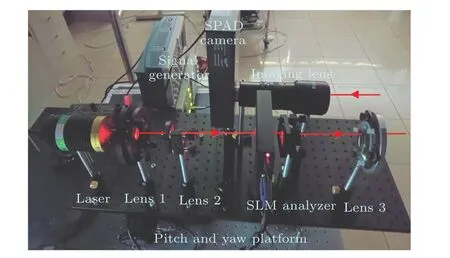
Fig. 6. Photon counting LiDAR system with spatially modulated illumination.

Table 1. System parameters.
Figure 7 shows the curve of the received signal photon number versus the SLM gray value at pixel (5, 6). For each pixel, an exponential function, such as formula (10) is used to fit the received signal photon number versus the SLM gray value
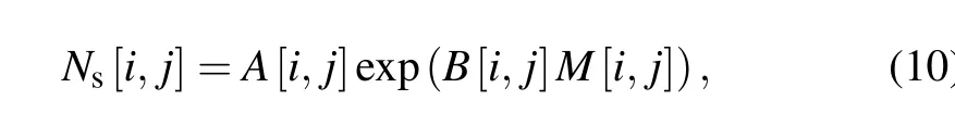
whereNs[i,j]is the number of received signal photons.A[i,j]andB[i,j] are the fitting parameters. Then, the gray valueM[i,j] can be calculated by substituting the required number of received signal photonsNs[i,j]=Nsetinto the inverse function of formula (10). The dynamic range of the combination of SLM and analyzer,can be calculated using the curve of the received signal photon number versus the SLM gray value.From the two adjacent pixels,the ratio between the minimum received signal photon number and the maximum received signal photon number is 0.11. The factors affecting this value include the extinction ratio of the analyzer and the degree of linear polarization of the laser.
Figure 8 shows the modulation matrix of the SLM under various preset average numbersNsetof signal photons at each pixel. Pixels that appear as white dots in Fig.8 are called hot pixels.A small number of hot pixels in the SPAD camera have abnormally high dark count rates due to imperfect fabrication,which results in large ranging and intensity errors. Hot pixels can be removed using noise-filtering operations.
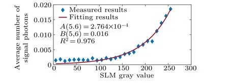
Fig.7. Curve of received signal photon number versus SLM gray value at pixel(5,6). The goodness of fit R2=0.976.
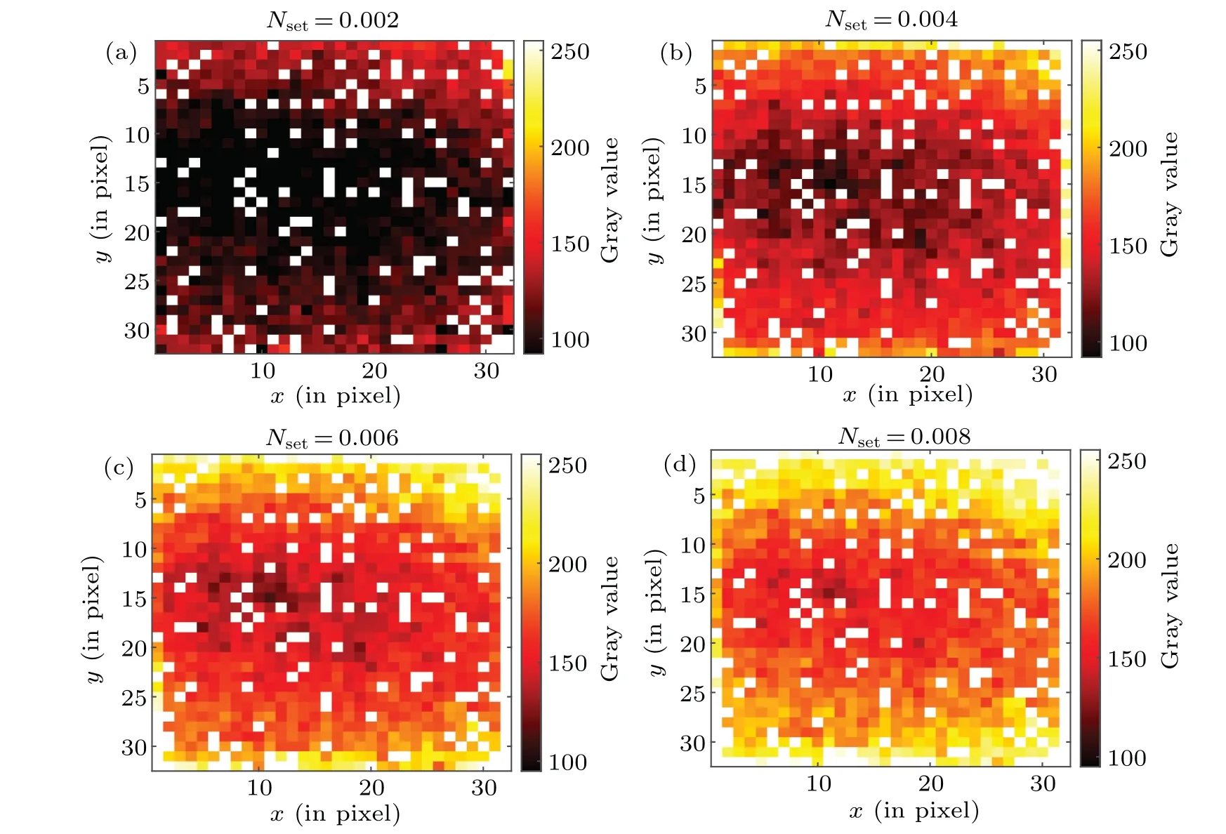
Fig.8. Modulation matrix of the SLM under various set average number of signal photons at each pixel. The average number of signal photons is(a)0.002,(b)0.004,(c)0.006 and(d)0.008.
We performed an experiment to image a white wall, as depicted in Fig.9(a),using the unmodulated method and proposed method. The SLM was not removed from the setup for the “unmodulated” measurements. Figure 9 shows the experimental results for the intensity images. Through 5×5 scanning, we stitched an image of 160×160 pixels. The distance between the system and objects was 4.27 m,and the total imaging FOV at the object plane was 0.76 m×0.76 m. Some cracks occurred in the adjacent stitching part of the image,owing to the alignment and resolution of the stepping of the pitch and yaw platform.This problem can be resolved by increasing the number of camera pixels to get rid of scanning or further modification with customized optical system and 2-axis Galvo scanning. The intensity image was obtained by summing the number of signal photons for each pixel. Owing to the direct illumination with the laser diode, the intensity image of each scanning block of the unmodulated method presented a pattern of strong middle and weak sides, as shown in Fig. 9(b).The standard deviation of the normalized intensity image depicted in Fig.9(b)is 0.109.The standard deviation of intensity was calculated over the full 160×160 pixels. Figures 9(d)and 9(e) show the experimental results of the proposed method.The quality reduction of the intensity image caused by the non-uniform illumination beam and non-uniform quantum efficiency of the detector array was improved through spatially modulated illumination. For the proposed method, the standard deviation of the normalized intensity image was reduced to 0.089. In order to intuitively compare the results of the two methods, Figs. 9(c) and 9(e) demonstrate the intensity profile slices across thexdirection of the two methods, wherex=0.076 m andy=0-0.152 m.
Other experiments were performed to image a scene, as shown in Fig.10(a). The scene comprises a cone,lamp,doll,and suitcase. All objects were placed on a table. These experiments were conducted to compare the performances of the unmodulated and proposed methods.The stand-off distance of the scenes was 4.27 m.The exposure time of the SPAD camera was 100 µs per frame, and 20000 laser pulses were accumulated to obtain a 32×32 photon-counting histogram. The total acquisition time for a complete 160×160 pixel image was 62 s.Because the scanning is the movement of the pitch and yaw platform with the entire imaging system,the scanning speed is not set fast.In the future,faster imaging speed can be achieved through optical system integration and 2-axis Galvo scanning system. The experimental environment in Fig.10 is closed indoor with lights off during the daytime. In these experiments,the average number of background noise per pixel per laser cycle was 0.1183. A natural scene has many details. The intensity image of the unmodulated method was superimposed with additional non-uniform noise, as shown in Fig. 10(b), which hindered subsequent noise filtering and target recognition.The intensity image of the proposed method is shown in Fig.10(e).The extra lateral noise was eliminated by spatially modulated illumination,which makes the intensity image more similar to the real situation. The depth image was calculated using the cross-correlation method. The hot pixels in the camera were simply filtered out through median filtering. The depth image results are shown in Figs.10(c)and 10(f). The objects maintained good outlines and details, except for a few areas with low intensity and no signal. The unmodulated method had the same depth image quality as that of the proposed method.Figures 10(d) and 10(g) show the 3D images that combine the intensity and depth images to intuitively demonstrate the imaging results. In this experiment, the average number of signal photons in the proposed method and the unmodulated method were 0.0047 and 0.0054,respectively. Due to lack of the ground truth,we calculated the SNR[29]for each intensity image for comparison quantitatively. The SNR was calculated by using SNR=|〈I1〉-〈I2〉|/((σ1+σ2)/2), where〈I1〉and〈I2〉are the average intensities calculated within the dashed black square and dashed white square in Fig.10.σ1andσ2are the standard deviations of the intensities in the dashed black square and dashed white square respectively. The SNRs calculated of Figs.10(b)and 10(e)were 1.86 and 1.24.Because a small number of pixels had abnormally high count rates in the reconstructed image of proposed method,the calculated SNR of the proposed method was lower than that of the unmodulated method.
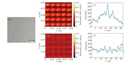
Fig.9. Experimental results of a white wall. (a)RGB photograph of the scene. (b)Intensity image of the unmodulated method. (c)Intensity profile slice across the x direction of the unmodulated method. x=0.076 m and y=0-0.152 m. (d)Intensity image of the proposed method. (e)Intensity profile slice across the x direction of the proposed method. x=0.076 m and y=0-0.152 m.
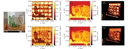
Fig.10. Experimental results of multiple objects. (a)RGB photograph of the scene. (b)Intensity image of the unmodulated method. (c)Depth image of the unmodulated method. (d)Three-dimensional demonstration of the reconstructed result from the unmodulated method. (e)Intensity image of the proposed method. (f)Depth image of the proposed method. (g)Three-dimensional demonstration of the reconstructed result from the proposed method.
Other experiments were carried out to test the performance of the unmodulated method, soft normalization method, and the proposed method in an environment with a stronger noise background. As exhibited in Fig.11(a),the image scene includes a cone,blanket with circle pattern,doll,and an‘8’-shaped foam board. All objects were placed on a table.The stand-off distance of the scenes was 4.27 m. The total acquisition time was the same as that in the experiment shown in Fig. 10, which was 62 s. We injected extraneous ambient light using a fluorescent lamp for the measurements shown in Figs.11(b)-11(d). In these experiments, the average number of background noise per pixel per laser cycle was 0.2229.Two fluorescent lamps were used to inject extraneous ambient light,as shown in Figs.11(e)-11(g). In these experiments,the average number of background noise per pixel per laser cycle was 0.4437. The intensity image of the unmodulated method was still superimposed with additional lateral noise,as shown in Figs. 11(b) and 11(e). The soft normalization method divided the captured normalized intensity image by the white wall normalized intensity image depicted in Fig.9(b)to remove the additional lateral noise. Compared with the unmodulated method, the soft normalization method improves image quality. However, according to the Poisson detection process, the lateral noise of the intensity image collected at a certain time will not have a one-to-one correspondence to that of the intensity image depicted in Fig.9(b). A simple division still produces additional lateral noise, particularly with high ambient noise, as shown in Figs. 11(c) and 11(f). The intensity images of the proposed method are shown in Figs. 11(d)and 11(g). The extra lateral noise was effectively eliminated by spatially modulated illumination. The SNRs calculated of Fig.11 were(b)6.70,(c)6.61,(d)7.26,(e)5.85,(f)3.58 and(g)5.20,respectively. Using a power meter,we measured the optical power used to illuminate the scene in Figs.10 and 11 as 30.2µW with the unmodulated method. The optical power emitted from the laser was 4 mW. After lens 2, the optical power decreased to 2.3 mW.Then,the optical power transmitted from the SLM was 605 µW. After the analyzer, the optical power was 43.1µW.For the proposed method,the optical power transmitted from the SLM was 603 µW and became 32.1µW after the analyzer. The optical power used to illuminate the scenes in Figs.10 and 11 was 22.8µW.The transmittance of the analyzer was the lowest among all the systems. It is necessary to improve the transmittance of the analyzer for practical applications. By measuring two white plane objects with varying intervals, it was found that the depth resolution of the system was 2 cm.
By performing TV-regularized denoising minimization on the intensity images in Figs. 11(e)-11(g), the denoising results were obtained, as shown in Fig. 12. A CVX tool for specifying and solving convex programs[30,31]helped solve the problem in Eq. (7). Owing to the existence of additional lateral noise,the denoising result of the unmodulated method was still noisy with the same pattern depicted in Fig.9(b).Figure 12(b)shows the noise reduction results of the intensity image in Fig.11(f). Additional lateral noise was mistakenly retained as the estimated intensity image of the scene. We could not identify any information concerning the real object’s intensity from the noise reduction results. Because the proposed method could effectively remove additional lateral noise, the denoised intensity image using the TV-regularized minimization method had a satisfactory quality. The TV-regularized denoising method not only removes the random noise but also maintains a clear edge of the object. The SNRs calculated of Figs.12(a), 12(b)and 12(c)were 10.77, 10.32 and 26.14, respectively. With the help of the TV-regularized denoising,the SNR of the intensity image of the proposed method was significantly improved.
Considering the appropriateness of memory consumption, the image was quartered before TV minimization denoising, and only one part was processed at a time. Finally,the four estimated results were stitched together to obtain a full-size image.There were two discontinuous lines caused by step-by-step optimization and splicing, as shown in Fig. 12.These discontinuous lines were mainly caused by the discontinuity in the calculation of the total variation at the outer edge of the four sub-parts. We used a basic TV-regularized denoising method to demonstrate the improvement of the proposed method on the denoising process in single-photon imaging. It is worth mentioning that the TV-regularized denoising method maintains a clear edge of the object but induces the staircase effect.[32,33]The most obvious example is the creation of image flat areas separated by boundaries when denoising a smooth ramp. The intensity images of the objects used in the experiments have few ramps,so the staircase effect can be ignored. Hybrid penalty denoising method such as the combination of waveletl1-norm and total variation[34]can be used to suppress the staircase effect.

Fig.11. Experimental results of multiple objects under two ambient noise conditions. (a)RGB photograph of the scene. (b)-(d)Intensity images using the unmodulated method,soft normalization method and proposed method with an average background noise count of 0.2229 per pixel per laser cycle.(e)-(g)Intensity images using the unmodulated method, soft normalization method and proposed method with an average background noise count of 0.4437 per pixel per laser cycle.
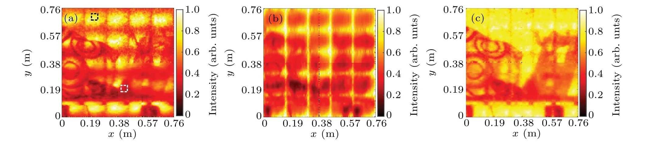
Fig.12. Noise reduction results for the intensity images of multiple objects. (a)Noise reduction result of the unmodulated method. (b)Noise reduction result of the soft normalization method. (c)Noise reduction result of the proposed method.
5. Conclusion
Photon-counting LiDAR using a 2D array detector has the advantages of high lateral resolution and fast acquisition speed. Two-dimensional array photon-counting LiDAR requires the use of floodlight to illuminate the scene. The non-uniform intensity profile of the illumination beam introduces additional lateral errors in the intensity image. The nonuniformity such as quantum efficiency and noise characteristics of the 2D array detector would degrade the image quality as well. Therefore,subsequent image noise reduction,and target recognition are significantly hindered. In this study, we propose a photon-counting LiDAR system that uses a spatial light modulator in the illumination channel to control the spatial intensity of the illuminating beam across a scene being imaged onto a 32×32 pixel photon-counting detector array.By controlling the spatial intensity to compensate for both the non-uniform intensity profile of the illumination beam and the variation in the quantum efficiency of the detectors in the 2D array, accurate intensity images can be obtained. LiDAR systems that employ avalanche photodiodes or conventional photodiode arrays face the same problem caused by the nonuniform illumination beam and the performance difference of the detector array. The proposed method is also applicable to these LiDAR systems. In the future, it will be of interest to further modify the system with customized optical system and 2-axis Galvo scanning. Optimizing the system to deal with a more complex imaging environment will also be considered.
猜你喜欢
学苑创造·A版(2022年4期)2022-06-18
文萃报·周二版(2022年18期)2022-05-11
作文大王·低年级(2022年2期)2022-02-28
东坡赤壁诗词(2020年2期)2020-06-04
东坡赤壁诗词(2019年3期)2019-07-05
红土地(2019年1期)2019-04-25
华人时刊(2018年15期)2018-11-10
景德镇陶瓷(2017年3期)2017-08-18
数学大王·低年级(2016年8期)2016-05-14
数学大王·低年级(2016年6期)2016-05-14

- Chinese Physics B的其它文章
- Characterizing entanglement in non-Hermitian chaotic systems via out-of-time ordered correlators
- Steering quantum nonlocalities of quantum dot system suffering from decoherence
- Probabilistic quantum teleportation of shared quantum secret
- Spin–orbit coupling adjusting topological superfluid of mass-imbalanced Fermi gas
- Improvement of a continuous-variable measurement-device-independent quantum key distribution system via quantum scissors
- An overview of quantum error mitigation formulas