
Rolling velocity and relative motion of particle detector in local granular flow
2022-11-21 09:29RanLi李然BaoLinLiu刘宝林GangZheng郑刚andHuiYang杨晖
Chinese Physics B 2022年11期
Ran Li(李然) Bao-Lin Liu(刘宝林) Gang Zheng(郑刚) and Hui Yang(杨晖)
1School of Health Science and Engineering,University of Shanghai for Science and Technology,Shanghai 200093,China
2School of Optical-Electrical and Computer Engineering,University of Shanghai for Science and Technology,Shanghai 200093,China
The velocity of a particle detector in granular flow can be regarded as the combination of rolling and sliding velocities.The study of the contribution of rolling velocity and sliding velocity provides a new explanation to the relative motion between the detector and the local granular flow. In this study, a spherical detector using embedded inertial navigation technology is placed in the chute granular flow to study the movement of the detector relative to the granular flow. It is shown by particle image velocimetry(PIV)that the velocity of chute granular flow conforms to Silbert’s formula. And the velocity of the detector is greater than that of the granular flow around it. By decomposing the velocity into sliding and rolling velocity,it is indicated that the movement of the detector relative to the granular flow is mainly caused by rolling.The rolling detail shown by DEM simulation leads to two potential mechanisms based on the position and drive of the detector.
Keywords: local velocity distribution,rolling velocity,inertial navigation technology,relative velocity dependent(RVD)rolling friction
1. Introduction
Traditional granular flow velocity distribution is studied usually[1]by using the monodisperse granular flow for the exploration of flow models[2,3]while the the research of polydisperse particle flow focuses on the mechanism of mixing and segregation.[4,5]However, there is a special particle flow of a few special particles worthy of attention in the nearly monodisperse granular flow,e.g.,rock landslides with accompanying debris flows are examples of such particle flows.[6]The number of special particles cannot form the statistical characteristics to support the segregation and mixing model exploration. The description of the movement of the special particles relative to the granular flow is very lacking. This process can be studied by placing inertial navigation detector into the chute granular flow,which can provide a valuable reference for the study of the movement process of special particles.
In the absence of a unified framework,granular flows in a chute are commonly divided into three different regimes based on the inertial number.[7]This study focuses on the viscouslike regime. The material flow is more like a liquid with a shear-rate-dependent stress under this regime.[8]
The local rheology is the most widely recognized mathematical model for viscous-like granular flow in an inclined chute.[9,10]Forterre and Pouliquen[11]and Tripathi and Khakha[12]summarized the local flow velocity distribution model as shown in Fig. 1(a). A granular layer of thicknesshflows down a rough plane inclined at an angle 8°<θ <12°.The force balance for steady uniform flows implies that the ratio between shear stress and normal stress is constant and equal to tanθ. Experimentally or numerically, the mean velocity varies as the power 3/2 of the depth and increases with inclination. The physical mechanism is the nonlinear correlation between the friction coefficientμand the inertial numberI[7,9]in the quasi static and kinetic regime,specifically

which is shown in Fig.1(b).
However,this model does not distinguish between the velocity caused by particle sliding and that by particle rolling.The latest research shows that rolling has an important influence on the movement of granular flow.[13,14]
Wanget al. reported a study on the granular flow layers by using the embedded inertial navigation techniques.[15]This provides a new method of studying particle rolling in a particle flow. Caviezelet al.studied rockfall on Alps by using a detector equipped with a situ sensor,and successfully reconstructed the falling trajectory of the detector.[16,17]Zhuet al.improved the navigation techniques and applied them to the study of the funnel flow particle rolling in the laboratory, and accurately measured the angular velocity distribution of the tracer particles in the funnel flow.[18]It was found that there is a close relationship between rolling and the granular flow velocity distribution. This provides an important reference for the study of the relative particle flow motion of special particles.

Fig.1. Local flow velocity distribution in chute granular flow:(a)schematic diagram of flat inclined chute and(b)nonlinear correlation between friction coefficient and inertial number.[11,12]
It should be noted that the PIV method and the xray method will not interfere with the particle flow and are a reliable method to measure the particle flow velocity distribution.[19]Since x-ray may offset the inertial navigation device,the PIV is chosen to measure the velocity distribution of chute granular flow which is used as the baseline. However,there are physical parameters which cannot be obtained by the experimental technology. With the development of computer technology, the discrete element method (DEM) is increasingly used in the granular flow mechanism research field.[20,21]The DEM can track the real-time motion of each particle,and obtain the particle’s rotational motion information.[22]The influence of rolling friction coefficient was investigated in Yu and Saxen’s DEM study of Silo.[23]Tripathiet al.adopted the relative velocity dependent(RVD)rolling friction in quantitative DEM simulation of non-spherical particle.[24]Taking the rolling friction into consideration in the model,the consistency of simulation results and experimental results is improved.
In this work,the data obtained from DEM simulation validated by spherical detector experiments are used to study the local granular flow,attempting to identify the velocity of particle as the rolling and sliding velocity in local flow velocity so as to provide a new perspective for the study of the movement of special particles relative to granular flow.
2. Experimental setups
2.1. Chute granular flow
Based on the theoretical model,the experimental process in this study can be seen in Fig. 2. The chute granular flow lasted 2.7 s on average and 2.8 s in this experiment served as an example. Att0=0,the baffle is removed and the particles started to move. The velocity distribution is unstable initially but att1=0.6 s, the chute granular flow forms a stable local flow velocity distribution. Aftert2=1.2 s,owing to the inadequate thickness of the particle bed in the chute,the local flow velocity distribution cannot be maintained.
We use the PIV technique to obtain the velocity on the side wall of the chute, as shown in Fig. 2(d). The detector is used as the special particle of concern (diameter of 30 mm),surrounded by small particles(diameter of 10 mm)inside the chute. The spherical detector can obtain the particle’s acceleration and rotation angular velocity. Therefore, the particle velocities of different initial heights in the chute and the composition of particle velocity under different inclination angles are studied.The position of the spherical detector isZ1,Z2,Z3,...,Z6, with a spacing of 15 mm. The thickness of the filled particles in the chute is 110 mm. The diameter of the filled particles is 10 mm,and the diameter of the spherical detector is 30 mm. To ensure that the velocity of the bottom particle is 0,a rough surface with a coefficient of friction of 0.8 is set as the bottom of the chute. More detailed description of the system is given in Refs.[14,15].

Fig. 2. Snapshots of chute granular flow, showing granular profile at (a)t0 =0, (b)t1 =0.6 s, chute granular flow formed stable local flow velocity distribution;(c)after t2=1.2 s,local flow velocity distribution failing to be maintained due to the inadequate thickness of the particle bed in the chute;(d)example displaying the granular flow at t=1 s to show the PIV measurement results.
2.2. Spherical detector based on embedded inertial navigation technology
The spherical detector is used to measure the angular velocity,acceleration and other movement data during the experiment through using embedded inertial navigation technology.
Any attitude in three-dimensional space can be represented concisely, intuitively by Euler angles. The aerial sequential Euler angles (shown in Fig. 3(a)) are used to represent the attitude of spherical detectors,φ,χ,Ψ, respectively,as the roll angle,pitch angle,and yaw angle. In the carrier coordinate system of the spherical detector,xbmoves to the right along the horizontal axis,ybmoves forward along the longitudinal axis,andzbmoves along the vertical axis. In the spatial coordinate system (E),xEis the projection ofxbon the horizontal plane,yEis perpendicular toxE,andzEis perpendicular to the horizontal plane.
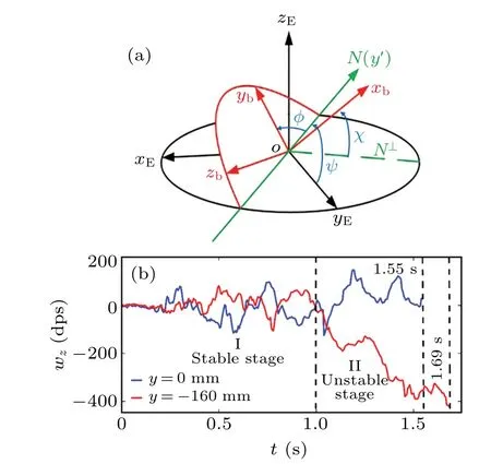
Fig. 3. (a) Schematic diagram of attitude angle of spherical detector, with ω′x,ω′y,ω′z,respectively,representing the components of original angular velocity of rolling around the x axis,y axis,and z axis,and ωy being the angular velocity of rolling around the y axis; (b) results from a typical experiment with two detectors placed side by side at Z1.[14,15]
The Euler angle is adopted in the measurement system to represent the attitude,and a quaternion is used to represent the attitude when it is solved.[25,26]The attitude update equation of the inertial measurement unit(ωx,ωy,andωzare the values that are measured by the gyroscope)is given as follows:

whereqis the quaternion expression.Nis the unit matrix,Ωnnbis the skew matrix of angular velocity, andTis the time interval.
Therefore, the attitude of the spherical detector is converted into a quaternion representation through the following equation during the attitude solution:
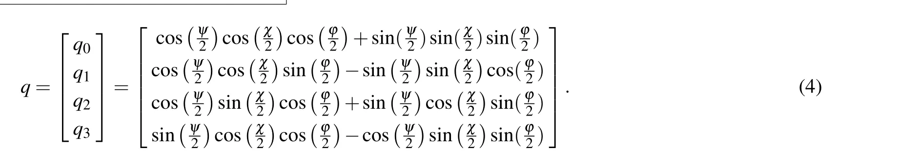
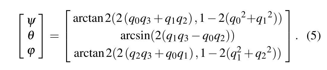
After the attitude solution is completed, the attitude is converted into Euler angles throughthe following equation:
Through multiple experiments, the experimental results of spherical particle wireless measurement technology based on inertial navigation technology are validated and can be used to measure the angular velocity and translational velocity of particles in the chute system.[15,18]
Figure 3(b)shows a typical experimental results obtained by using two spherical detectors placed atZ1. It can be found that the movement process of the detectors can be divided into stable stage and unstable stage by the rotating speed.[14]To discuss the rolling and sliding of the detector,we focus on the relationship between the particle flow velocity distribution and the special tracer particle velocity characteristic from 0.6 s to 1 s(stable stage).
2.3. DEM simulation
2.3.1. DEM contact model
The most important step in DEM is to choose a reasonable physical contact model. The model of Hertz–Mindlin(no slip)with RVD rolling friction adjusts the calculation method of rolling friction to ensure that three dimensions have the proper functionality without affecting the calculation time. It is especially suitable for strong rotation systems that have strict requirements for particle rotation characteristics.[24]Therefore,in this paper DEM is used based on the model of the Hertz–Mindlin(no slip)with RVD rolling friction contact to simulate the discharge process of spherical particles in a chute.According to the relative rotational velocity between contact particles,the particle rolling friction is calculated as follows:[27]

where torqueτrepresents the rolling friction of the particles,μris the rolling friction coefficient,Fnis the normal force between particles,R*is the equivalent radius between particles, ˆωrelis the unit vector of relative rotational velocity,E*is the equivalent Young’s modulus,andδnis the normal overlap amount.
The equivalent radiusR*and the equivalent Young’s modulusE*are calculated from the following equations:

whereiandjrepresent the two particles in contact,RiandRjare the radii of the contact particles,viandvjare the Poisson’s ratio,EiandEjare the Young’s moduli.
2.3.2. Simulation setup
Figure 4(a)shows the theoretical model of chute flow defined three layers based on the velocity distribution.[28]The experimental results presented in Ref. [15] indicate that the rolling contribution rate is an important factor affecting velocity composition.Figure 4(b)shows the simulation chute crosssectional surface sliced into 30×60 grids,and each grid is the smallest statistical unit with a size of 10 mm×20 mm×10 mm.In the simulation, the average movement information of the particles in each grid is used. The simulation process is the same as the experimental process shown in Fig. 2. Three particles (d= 1 cm) in each layer are marked. A detector(d=3 cm)is placed in the granular bed atZpoint,near particle B.
During the simulation,the time interval for collecting particle motion data is set to be 0.01 s. In order to ensure the stability of experiment,the minimum time step in experiment is set to be 2.71×10⁻⁵s,which is less than the Rayleigh time of particle 5.82×10⁻⁵s.[29]Other system parameters of DEM simulation are shown in Table 1.
Among them, the friction coefficient between particlesμp-pis obtained by measuring the repose angle of particle accumulation, and the coefficient of restitutioneis obtained by the particle rebound experiment.[30]
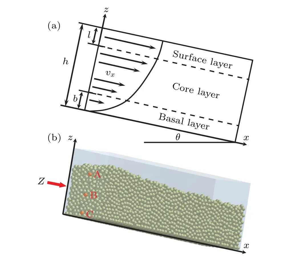
Fig.4. Simulation based on the velocity layers: (a)schematic model of the chute system and(b)geometry of chute with an initial packed bed.
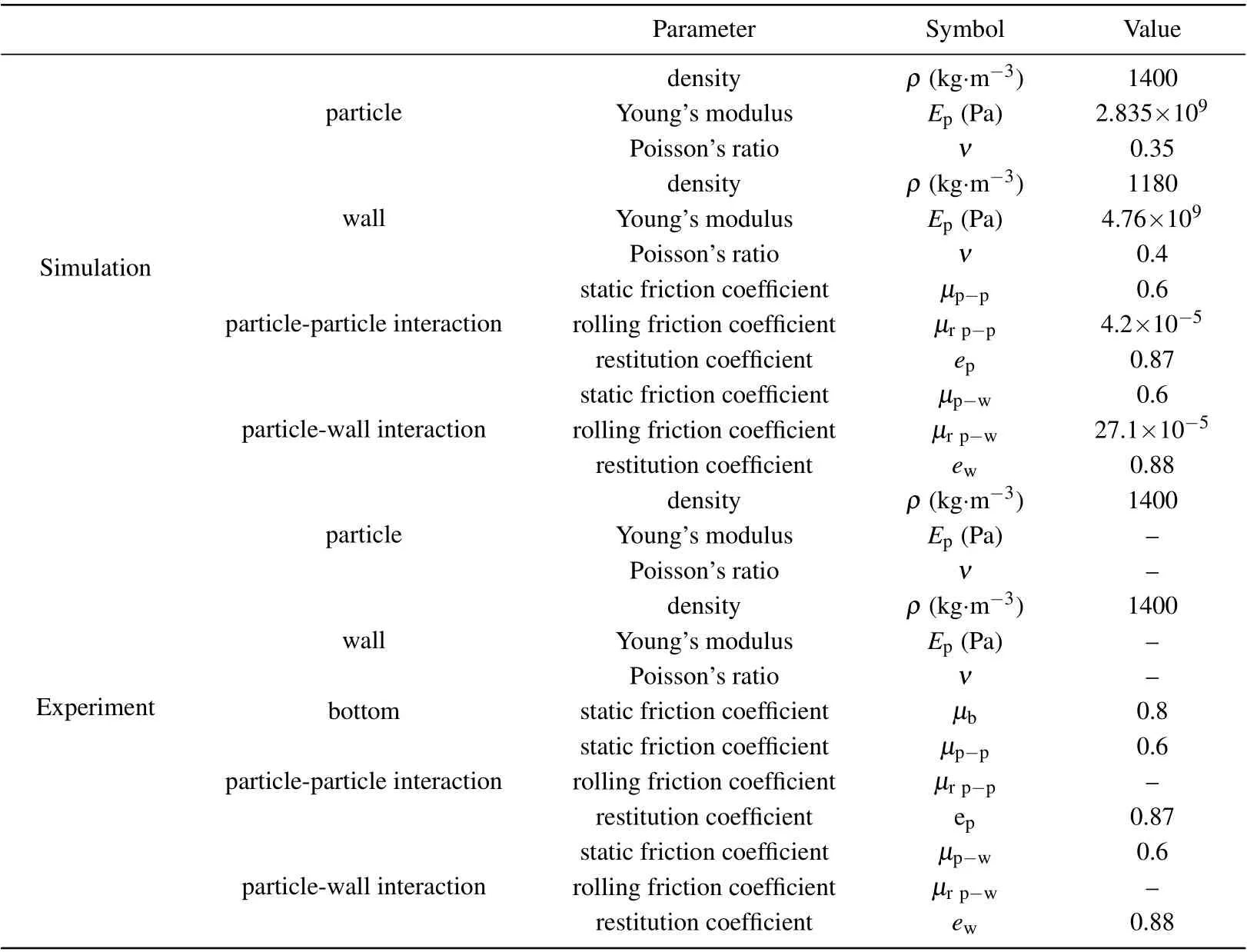
Table 1. Physical parameters employed in experiments and simulations.
3. Results and discussion
3.1. Relative motion between detector and granular flow
In the local granular flow model, it is believed that the flow velocityvx(z)is positively correlated withz3/2. The relationship between the flow velocity and the height of the chute can be expressed as(also known as Silbert’s formula)[7]
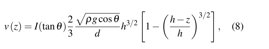
whereIis the inertial number which increases with inclination angleθ, increasing,his the thickness of the filling particle,ρis the density of the filling particle,gis the acceleration of gravity,θis the angle between the chute and the ground,andzis the height of the chute. Based on Eq.(8),the calculated velocity of the granular flow is shown by the red line in Fig.5(a)whenθis 12°.

Fig.5.(a)Comparison between theoretical curve and experimental curve of,chute height versus particle flow velocity,with red line representing velocity based on Eq.(8),where I=0.178,black line denoting averaged velocity measured by PIV method. and blue triangles referring to the velocities measured by using a spherical detector at six marked locations;and(b)curve of chute height versus relative velocity between the detector and the granular flow.
We use the PIV method to obtain the averaged velocity profile on the side wall of the chute,and the detector to obtain the average velocity of special tracer particle during the stable period. It is shown in Fig.5(a)that the averaged velocity measured by the PIV method is similar to that obtained from the theoretical model,Eq.(8).The red line shows that the granular velocity at the bottom is not 0,whereas in Eq.(8)the grain at the bottom should not slip. This is because the chute does not use particle bed as bottom,so the granular layer at the bottom does not form complete stable state.
The velocity measured by the detector at different values ofh(as shown by the blue points)is larger than the PIV results and increases linearly. This indicates that the detector moves faster than the surrounding particles. The relative velocity between the detector and the granular flow is shown by Fig.5(b).The biggest difference in velocity appears at the bottom.
3.2. Rolling velocity and sliding velocity
During the experiment, it can be observed in Fig. 2 that the particles in the chute have not only sliding motion, but also rolling motion. The velocity of the spherical detector is a combination of sliding velocity and rolling velocity as shown in Fig.6.
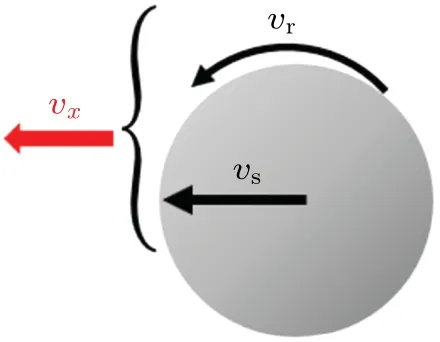
Fig.6. Composition of velocity: sliding velocity vs and rolling velocity vr.
The velocity along the flow directionvx(z)of the spherical detector can be expressed as
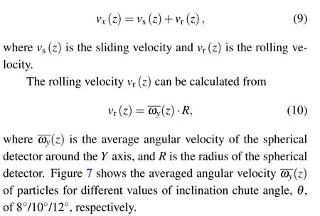

Fig.7. Curves of chute height versus averaged angular veloci(z)of the spherical detector at different inclination angles.
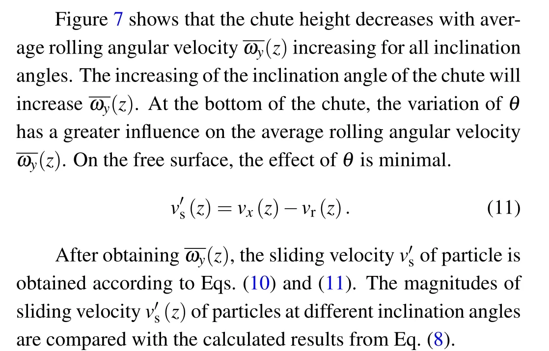
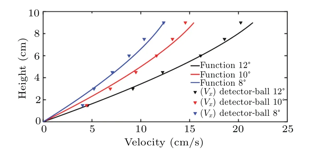
Fig. 8. Comparison of particle sliding velocity vs(z) among different values of inclination angle θ,with solid lines representing velocities calculated from Eq.(8),triangles denoting velocities measured by the spherical detector. Inertial number I =0.178 when θ =12°, I =0.140 when θ =10°.I=0.125 when θ =8°.
As shown in Fig. 8, the sliding velocities measured by detector and calculated from Eq.(8)are matched. At the free surface of the chute,the growth pattern of particle sliding velocityvs(z)tends to be flat. This is one of the characteristics of the local flow model,indicating that the sliding velocity of the detector is mainly driven by the local granular flow. Correspondingly, the velocity of the detector relative to the surrounding particles is mainly due to rolling.
3.3. Relative motion based on simulation results
Using the detector and PIV technology,the measurement results show that rolling and relative motion are statistically correlated. For further investigation,the results obtained from the DEM simulation (Fig. 4) are analyzed. The area in the middle of the chute is considered as the area that contains valid granular flow velocity distribution as shown in the inset of Fig.9. The velocities of each particle are shown by the black triangles. Calculations from Eq. (8) are shown by the red line. It can be observed that the simulation results are in line with the experimental results as shown by the blue line(the same as the red line in Fig. 5). The slight difference inIbetween 0.178 in experiment result and 0.182 in simulation result may be due to the ideal shear process obtained by simulation.
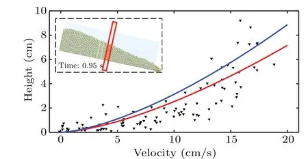
Fig. 9. Simulated velocity distributions, with inset showing measured area,triangles representing velocities of particles in measured area,red line(I =0.182) and blue line (I =0.178) denoting calculations from Eq. (8)based on the simulation and the experimental results.
By tracking the labeled particles, simulation results provide the accurate trajectories and real-time rolling velocities that cannot be obtained experimentally.
Figure 10(a)shows the rolling velocities of 3 labeled particles. The rolling velocity of particle A is larger than those of the other two labeled particles. The velocityvxof particle A located in the surface layer (Fig. 4) is significantly higher than those in the other layers. It takes less than 2 s to move out of the chute. This is consistent with the theory presented in Subsection 3.1.
The velocityωyof particle B is slightly larger than that of particle C in the stable stage. After 1.5 s, the values ofωyof particles B and C are the same. By tracking the labeled particles, it is found that particle B falls in height as it follows granular flow and approaches to particle C in a time between 0.5 s and 1.5 s. This causes relative motion between particle B and the core layer. After 1.5 s, particles B and C follow similar trajectories moving out of the chute. So a similarωyis obtained.
Because of the difference invx, the particles in different layers have obvious relative motions. The relative motion trajectory is consistent with that of velocityωy.
Figure 10(b)shows time-dependentωyof the detector and particle B.The detector moves faster,leaving the chute 0.55 s earlier than particle B at a similar initial position. Comparing withωyin the moving duration,the rotation of the detector is more stable and larger than the particle B on average. Several larger pulses in red line indicate that particle B moves intensely when there is a gap.

Fig. 10. (a) Curve of time-dependent angular velocity ωy of particles A(blue line),B(red line),and C(black line)on surface,core,and basal layer.(b)Curve of time-dependent angular velocity ωy of detector(blue line)and particle B(red line)located at similar initial position.
Fig. 11. Two potential mechanisms of ωy of detector: (a) detector surrounded by granular flow; (b) detector driven by the unbalanced granular flow;(c)detector starting to surface the granular flow;(d)detector driven by gravity.
Based on theωy,two potential mechanisms of the detector rolling are presented in Fig. 11. During the stable stage,the detector is surrounded by the granular flow as shown in Fig. 11(a). Because of the difference invxat different values ofh,the detector rolls forward under the drive unbalanced granular flow as shown in Fig.11(b).
During the unstable stage, the upper part of the detector is not covered by the granular flow. Figure 11(c) shows the moment when the detector surfaces the granular flow. It can be observed thatvxbelow the detector is not uniform. At this stage, the detector is driven by gravity, moving to the region with highervx.
Further investigation of the detector trajectory shows that the mechanism ofωyof the detector is correlated with the layer at which the detector is located. In the surface and basal layer,the detector has a higher probability of moving upwards. The direction is similar to that shown in Fig. 11(d). In the core layer,the trajectory of the detector is very complex. The motion directions indicated by both mechanisms occur. The relationship between rolling mechanism and time-space will be the focus of further research.
4. Conclusions
We experimentally studied a special particle moving in the local granular flow and consider that the velocity of the special particle should be divided into sliding velocityvs(z)and rolling velocityvr(z). Ashincreases, the sliding velocityvs(z) of particles increases, but rolling velocityvr(z)decreases. The velocityvx(z) of particles presents a linear growth,andωy(z)can be obtained by a spherical detector,thus the rolling velocity of the particlevr(z)can be obtained. Two potential mechanisms ofωyare presented based on the DEM simulation with RVD rolling friction model,andωyof the detector changes in different flow stages and layers. In further studies, the relationship between mechanism ofωyand timespace of the detector needs to be analyzed precisely and compared with theoretical models.
Acknowledgements
We would like to express our gratitude to Prof. V.Zivkovic from Newcastle University for his careful guidance and help.
Project supported by the National Natural Science Foundation of China (Grant Nos. 11972212, 12072200, and 12002213).
猜你喜欢
广东教学报·教育综合(2022年49期)2022-04-27
考试与评价·七年级版(2021年2期)2021-08-14
农机质量与监督(2020年7期)2020-12-14
考试与评价·七年级版(2020年4期)2020-10-23
娃娃乐园·绘本(2020年9期)2020-09-28
中学生博览(2019年2期)2019-01-23
都市(2016年9期)2016-11-22
小小说月刊(2015年11期)2015-05-14
连环画报(2015年4期)2015-04-19
小小说月刊·下半月(2012年4期)2012-05-14

- Chinese Physics B的其它文章
- A design of resonant cavity with an improved coupling-adjusting mechanism for the W-band EPR spectrometer
- Photoreflectance system based on vacuum ultraviolet laser at 177.3 nm
- Topological photonic states in gyromagnetic photonic crystals:Physics,properties,and applications
- Structure of continuous matrix product operator for transverse field Ising model: An analytic and numerical study
- Riemann–Hilbert approach and N double-pole solutions for a nonlinear Schr¨odinger-type equation
- Diffusion dynamics in branched spherical structure