Full immersion measurement on the sound speed and attenuation of the abyssal silty-clay sediment in South China Sea

CAO Xinghui,QU Zhiguo,ZHEN Huancheng,CHENG Hui

(1.Xinjiang Institute of Technology,Akesu 843000,Xijiang,China;2.Institute of Deep-sea Science and Engineering,Chinese Academy of Sciences,Sanya 572000,Hainan,China)

Abstract:By using full-immersion transducer measurement(FITM),a broadband sound speed and attenuation measurement method is presented,which provides a way to obtain the sound speed and attenuation of ultrafine sediments(average particle size of 5.27µm and porosity of 79%)in laboratory.The dependence between sound speed and attenuation was compared with Kramers-Kronig relation for confirming the reliability of the in-lab measurement.Meanwhile,Hamilton classic curves indicate that the in-lab measurement results meet the speed-porosity relation,and the attenuation from the in-lab method is within the confidence interval of Hamilton curves.The sound speed and attenuation prediction curves of the effective density fluid model and the grain-shearing model are satisfied which also proves the accuracy and availability of the in-lab measurement method.

Key words:sediment;sound speed;attenuation;ultrafine;tube

0 Introduction

Acoustic parameters of marine sediments can provide a reference for the inversion of geoacoustic data[1],as well as predict the geotechnical properties of sediments,which helps to ascertain the relationship between the geotechnical and acoustic properties in marine exploration techniques[2],and verifies the accuracy of the acoustic prediction model in sediments[3-5].Sound speed and attenuation measurements of marine sediments samples are usually obtained through insitu pushcore by ROV or gravity corer.Researchers have developed a number of devices for the in-situ measurement of acoustic parameters.In 1962,equipped with an in-situ probe for the measurement of sediments from a depth of 338-1 235 m off the coast of San Diego,CA,USA,Trieste submarine completed the first in-situ measurements of deep sea sediments[6].Major concerns of the vital 1999 marine sediment test included acoustic backscattering,the penetration of sound waves into marine sediments,and the propagation of sound waves in marine sediments.In addition,hydrodynamics effects on the formation of marine sediments were also observed[7-8].In recent years,the ballast acoustic measurement system has been employed in the South China Sea for sediment analysis[9].Since the temperature,pressure,and water content remain stable during in-situ measurements,it is generally accepted that data from in-situ measurement are more accurate than in laboratory.However,in-situ measurements are quite expensive,and it is not realistic to perform in-situ measurements over large areas of the seafloor.Fortunately,benefited from suitable experimental conditions,accurate measurements can be conducted in laboratory.Furthermore,the disturbance of in-situ sediments by instruments used is inevitable,and there are no enough time waiting for the sediments from disturbance to stability.Thus,in-lab methods have gained more and more attention of researchers[10-11].

The vast expanse of the South China Sea,as well as the movement of sediments by ocean currents and the varying temperatures and pressures of the sediments,collectively leads to the complexity of the sediments in the South China Sea.Several scholars have implemented probe methods in laboratory measurements[9,12]and have tried to improve the accuracy of their sound speed and attenuation measurements[13].Sound speed and attenuation predication models can be used to analyze additional acoustic properties of the sediments and perform the inversion of the physical properties of the sediments.These prediction models include the Biot-Stoll model,the effective density fluid model(EDFM)[14],and the grain-shearing(GS)model[15].The applicability of the various prediction models has been validated by the inlab and in-situ sound speed and attenuation measurements[9,13].All the experiments conducted in laboratory used pushcore samples.

In this paper,sediments samples are from a depth of 2595 m in the northern part of the South China Sea.The sound speed and attenuation of this ultrafine silty clay sediment are measured by using the fullimmersion transducer measurement(FITM)with continuous pulse signals,and sound tube under laboratory conditions.The dispersion characteristics of the sound speed and attenuation of ultrafine silty clay sediments are analyzed in a broad frequency band.Two identical sets of sediment samples are prepared for the experiments.The full-immersion source and receiver transducers are in direct contact with the sediments.

A large-aperture,low sidelobe,plane transducer is used in the experiment.The beam width of the transducer is 5.8°and the sidelobes are as low as-17 dB,which effectively ensures the beam directivity and signal quality.In the sound tube,the sound waves incident onto the sediments from the full-immersion source transducers are directly received by the fullimmersion receiver,thus,the effect of the tube bottom on the sound wave penetrating into sediments is eliminated,and the use of a coupling medium between the tube bottom and the transducer is also avoided.The full-immersion transmitter and receiver with good response performance are used to measure the sound speed and attenuation in a broad frequencies band.The dispersion relationship of the sound speed and attenuation in the frequency band of 50-140 kHz is evaluated.The Kramers-Kronig relation verified the accuracy of the measured sound speed and attenuation.Meanwhile,the measured data are compared with the Hamilton classic curves,EDFM,and GS models,showing that the measured results are reliable.

1 Materials and Analytical Methods

1.1 The silty clay sediment samples

In August 2018,sediment samples were collected from a depth of 2 595 m in the northern part of the South China Sea by using a shipborne TV grab.The samples were loose sediments,which is different from the pushcore samples obtained by using the gravity sampler or ROV.These samples contain a very small amount of sandy particles with particle sizes of>62.5 μm.The measurement of the acoustic parameters requires that the sediments are well classified,so as to separate out any sandy particles.Since there are only low levels of organic matter and no shells in the deep sea,it is possible to obtain sound speed and attenuation in laboratory.In this study,according to standard GB/T 50123-1999[16],the sediments are air-dried and fully ground into a fine powder with a roller,and then soaked in and fully mixed with seawater.Since the volume of the boiled sediments increases and their characteristics changes completely,the method of driving out the bubbles by boiling sediments is abandoned.Sediments samples in tube need to remain motionless more than three months until the sediment thickness no longer drop down.

It should be noted that for the sediment samples,a flocculation structure can be formed by seawater;so the sediment will get a finite stiffness to generate shear waves.If fresh water is used instead of seawater,the physicochemical bonds would be destroyed and the mixture samples would become a suspension.The measured attenuation coefficients in the mixtures of non-flocculation and flocculation are significantly different,which has been confirmed by numerous experiments[17].The sand-silt-clay composition and median particle size of the samples are measured by using a QL-1076 laser particle size analyzer.Table 1 shows the volume distribution of the different particle sizes of the sediments.The measurement error of the particle size analysis is less than 2%,and the median particle diameter is 5.27 μm.This type of sediments is referred to as ultrafine silty clay sediments.

Table 1 Volume distribution of sediment particle size(where the cumulative volume distribution of D10=1.14 μm,D50=3.87 μm,D90=11.51 μm and D[4,3]=5.27 μm)

1.2 Porosity analysis

Firstly,the loose sediments collected by the TV grab needs air-drying and sampling.The agglomerated portions are thoroughly separated by soft rubber.The samples are evenly tiled to ensure uniform heating while in the dryer at 105°C for 24 hours.Thedried sediments are cooled to room temperature,weighed,poured into a dial beaker,mixed with an equal amount of water,stirred thoroughly and sealed,and then stored at room temperature for one month.Water continuously precipitates within the upper layer of the water-saturated sediments,and the thickness of the precipitated water layer is measured.When the thickness of the water layer has stabilized,the watersaturated sediments are considered to have reached a stable state.Four sets of samples are prepared following the above procedure.The measured porosities of the water-saturated sediments are 77%,77%,78%,and 79%.

1.3 Sound measurement tube device

In this study,both the transmitter and receiver are the wideband transducers with flat-frequency response,and the effective bandwidth of the 6 dB frequency response is 60 kHz.Although only the function of transmitter or the function of receiver is used in each test,the transmitting and receiving transducers can be switched to validate the results.This type of transducer is custom-made by Suzhou Sheng-Zhi-Yuan Electronic Technology Co.,Ltd.

The sediment samples are loose sediments obtained from a shipborne TV grab,rather than the pushcore samples obtained by a gravity sampler or ROV.For the in-lab measurement method,the transmitter is installed inside the sound tube(without cover and bottom)and the connection between the transmitter and the tube wall is tightly sealed.The sediment is in direct contact with the full-immersion transmitter and the states of the transmitter and the sediments remain stable during the sediment precipitation and stabilization processes,as well as while measuring which ensures minimal disturbance of the sediments(Fig.1).The measurement system consists of an acoustic power amplifier and an Agilent 33500B Series signal generator for generating continuous pulse wave.The transmitted and received waveforms are simultaneously acquired by using an Agilent DSO-X 3054A oscilloscope in the high-resolution mode at a sampling rate of 500 MHz.Planar transducers,including two transducers with bandwidths of 50-70 kHz,are used as the source and receiver.Two other transducers with bandwidths of 80-140 kHz are also used as the source and receiver.During the measurements,the fullimmersion receiver is inserted into the sediments from the top of tube,and continuous pulse wave is emitted by the full-immersion transmitter below.The sediment layer is 145 mm thick in the tube for the 80-140 kHz transducers and 190 mm thick in the tube for the 50-70 kHz transducers.The sound wave penetrates into the sediments and is received by the receiver.The oscilloscope simultaneously acquires the transmitted signal and the received signal in the 500 M high-resolution mode.In order to accurately calculate the travel time of sound wave in tube,the oscilloscope uses two channels to simultaneously acquire the transmitted signal and the received signal.Fig.2 shows the signals of the receiver.As shown in the figure,the signal-to-noise ratios of the received signals are good.Due to the broadband characteristics of the transducers,one transducer can directly measure both the sound travel time and the sound attenuation at multiple frequencies,therefore,the position of the fullimmersion transducer can remain unchanged during measurement,and there is no need to replace the transducers.Thus,the measurement error introduced by the disturbance of the sediments is avoided.

Fig.1 Diagram of the full-immersion transducer measurement(T is the transmitting transducer and R is the receiving transducer)

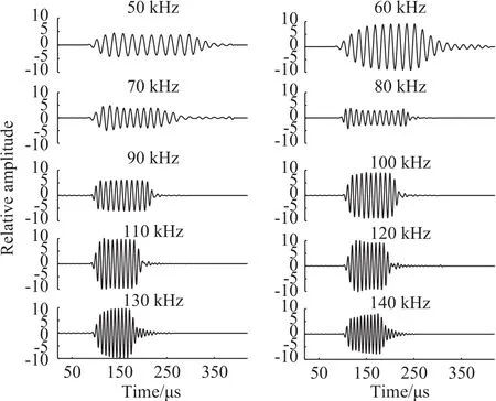
Fig.2 Received waveforms in the ultrafine sediment at different frequencies.

2 Calculation method

The calculation of the sound speed in the sediments is based on the travel time difference of the sound wave in the two media,and the sound attenuation calculation depends on the ratio of the received amplitudes in the two media.Fig.3 shows the received waveforms at 100 kHz.At the beginning and ending of the received waveform,the piezoelectric ceramic layer in the receiver is in the states of vibration start and vibration stop,respectively.The observed frequencies of the received waveform near these points observed by the oscilloscope deviate from the transmitted 100 kHz.In the medium part of the received waveform,the frequency is consistent with the transmitted 100 kHz.The time period in the start and the end of the waveform is referred to as the“response time”.The continuous pulse wave pulses must be wide enough to ensure that the waveform is received at accurate frequencies.

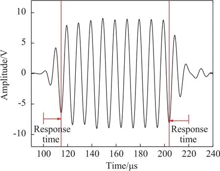
Fig.3 The 100 kHz waveform in sediments.The response times are defined by the beginning and ending sections of the waveform.The frequency of the middle section of the waveform is stable at 100 kHz.

For seawater in the first tube and for sediments in the second tube,the transmitted and received signals are recorded,respectively.Since high-frequency interference from the power amplifier affects the transmitted signal and the received signal,the interference components on the received signal need to be filtered out by a band-pass filter in advance.Then,the time difference between the signals to the receivers in the seawater and in the sediments is calculated the time difference Δt1.Since the two transmitted signals are not triggered at the same time,it is also necessary to calculate a time difference Δt2of signals emitting in the seawater and in the sediments.Therefore,the true time difference of the received signals in the two media is δt=(Δt1-Δt2).The relation of travelling time difference in seawater and sediments can be expressed as[18]

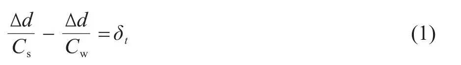
where Δd is the travel distance of the sound wave in sediments or seawater,Csis the speed of sound in the sediments,Cwis the speed of sound in the seawater,and δtis the travelling time difference in the seawater and the sediments.The sound speed Cwin seawater is measured by using the MINOS·X instrument.The frequency dependence of sound speed Csin the ultrafine sediments is obtained by Equation(1).

The peak amplitudes of the received signals in the seawater and the sediments are obtained after filtering,and the attenuation coefficient α(f)is calculated by the ratio of the peak amplitudes of the two received signals as shown in Equation(2)[19]:

where A(f)wis the peak-to-peak value of the re-ceived signals in the seawater,and A(f)sis the peakto-peak value of the received signals in the sediments.The dispersion relationship of the attenuation coefficient can also be obtained by Equation(2).

3 Results

3.1 Dispersion relationship of the sound speed

The dispersion relationship of the sound speed is shown in Fig.4,from which,it can be seen that the sound speed in the ultrafine sediments slowly increases with frequency in the range of 50-140 kHz,and the sound speed in is approximately 1480.9-1487.5 m/s in this frequency range.During the entire measurement process,the temperature varies between 27.6°C and 28.4°C;therefore,the effect of small changes in temperature on the sound speed is negligible.The linear fit of the data in Fig.4 shows a weak linear relationship between sound speed and frequency.The fitted curve is expressed as

Fig.4 Sound speeds of the ultrafine sediments at different frequencies in the ultrafine sediments and in a temperature range of 27.6-28.4°C

where f is the frequency in kHz,Csis the sound speed of the ultrafine sediments in m·s-1,and r is the correlation coefficient.Based on the equation,the sound speed in the ultrafine sediments has an average increase of 0.066 4 m·s-1·kHz-1in the 50-140 kHz frequency range.The results show that the sound speed in the ultrafine sediments is weakly correlated with frequency.

3.2 Frequency dependence of the attenuation

The frequency dependence of the attenuation of in the ultrafine sediments is shown in Fig.5.Within the 50-140 kHz frequency range,the attenuation coefficient of the ultrafine sediments changes from 4.02 to 25.11 dB·m-1,indicating a strong positive correlation within this frequency range.Hamilton compiled a large amount of in-situ and experimental data[17],and then determined that the dispersion relation of the attenuation coefficient can be expressed as

where α is the attenuation coefficient of the compressional waves in dB/m,f is the frequency in kHz,k is a constant,and n is the exponent of the frequency.For sediments with different physical properties,k and n are also different.Fig.5 shows three regression curves of attenuation coefficient versus frequency.The linear regression is expressed as follows:

The frequency dependence of the attenuation coefficient is better fitted by f2and the fitting equation is

Among the three fitting curves,the best-fit curve is

Based on Fig.5 and the correlation coefficients r in Equations(5),(6),and(7),it can be seen that the frequency dependence of the attenuation coefficient is better fitted by f2than f1in the range of 40-150 kHz.

Fig.5 Sound attenuation coefficients of the ultrafine sediments at different frequencies:The red solid line is the curve fitted by f2,and the red area is the confidence band of the f1fitting curve.The purple dashed line is the curve fitted by f2,and the blue area is the confidence band of the f2fitting curve.The black solid line is the fitted curve for the maximum r2,and the power exponent n of the frequency is 1.7

4 Discussions

4.1 Frequency dependence of the attenuation

Firstly the validity of the sound speed attenuation data is verified by the Kramers-Kronig relation.Mangulis was the first one to apply the Kramers-Kronig relation to the acoustics study[20].Based on the acoustic kk relation given by Mangulis,O’Donnell obtained the following localized expression from a mathematical transformation under the condition of a small dispersion[20]:

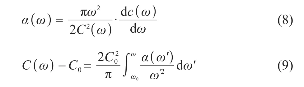
Here,C0is the sound speed in m·s-1,ω0in Hz,and the unit of α(ω)is Np·m-1(1 Np·m-1=8.686 dB·m-1).

This is a local approximation expression of the Kramers-Kronig relation.This approximation accurately describes the relationship between the frequency dependence of attenuation and sound speed dispersion,which has been demonstrated in solution and in the soft tissue animals[21].We select the data that satisfies the Kramers-Kronig approximate local expression,that is to say the linear data of frequency dependence of attenuation.So we can use the data to predict the sound speed in order to verify the sound speed data measured in laboratory[22-25].The predicted sound speed curve is calculated according to the attenuation curve in the frequency range.Then,the predicted sound speed is compared with the sound speed curve measured in the laboratory(Fig.6).

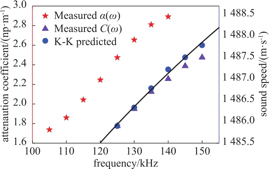
Fig.6 Comparison of the sound speed predicted by the k-k relation and the sound speed measured in laboratory.

As shown in Fig.6,by using the sound attenuation data obtained in the laboratory,the sound speed can be well predicted,showing that the experimental sound speed is reliable.In the high frequency range,the sound speed predicated by the Kramers-Kronig relation deviates from the measured sound speed due to the change in the linearity of the sound attenuation.

4.2 Comparison with the Hamilton data

First,we discuss the results of the sound speed of ultrafine sediments.Hamilton introduced the concept of sound speed ratio to measure the relationship between sound speeds of sediments and water,i.e.,the ratio of sound speed of sediments to sound speed of water[25].Hamilton determined that this ratio is consistent under in-situ and in-lab conditions.Shunway determined that porosity is the only most important factor causing changes in the compressional sound speed of loose sediments.This is due to the difference in the compressibility of water and mineral particles,so the porosity is an indicator of the relative fluid and solid contents[26].Shunway verified that the sound speed of high-porosity sediments is slightly lower than that of water[27].Hamilton concluded that the compressional sound speed of high-porosity sediments is usually less than that of water in the laboratory and field,and there is no speed dispersion within a very wide frequency range[17].

The relation between the sound speed ratio and the porosity determined by Hamilton is shown in Fig.7[27],in which the horizontal axis represents the percentage volume of solid.Hamilton provided the sound speed curve of typical sand-silt.The sound speed curve shows that as the particle concentration increases,the sound speed decreases by about 4% until the concentration reaches 20%,after that it gradually increases.Above 46%,the sound speed ratio is greater than 1.0.The porosity of the ultrafine sediments in our experiment is 79%,i.e.the percentage volume of solid is 21%,and the corresponding sound speed ratios of 0.972-0.976 are calculated at 22.8°C,which are indicated by red triangles in Fig.7.The sound speed ratios of the ultrafine sediments measured in the laboratory agree well with the Hamilton’s curve.Moreover,Fig.7 also shows a good agreement with the sound speed ratio obtained by an in-situ measurement of sediments in the South China Sea[28].

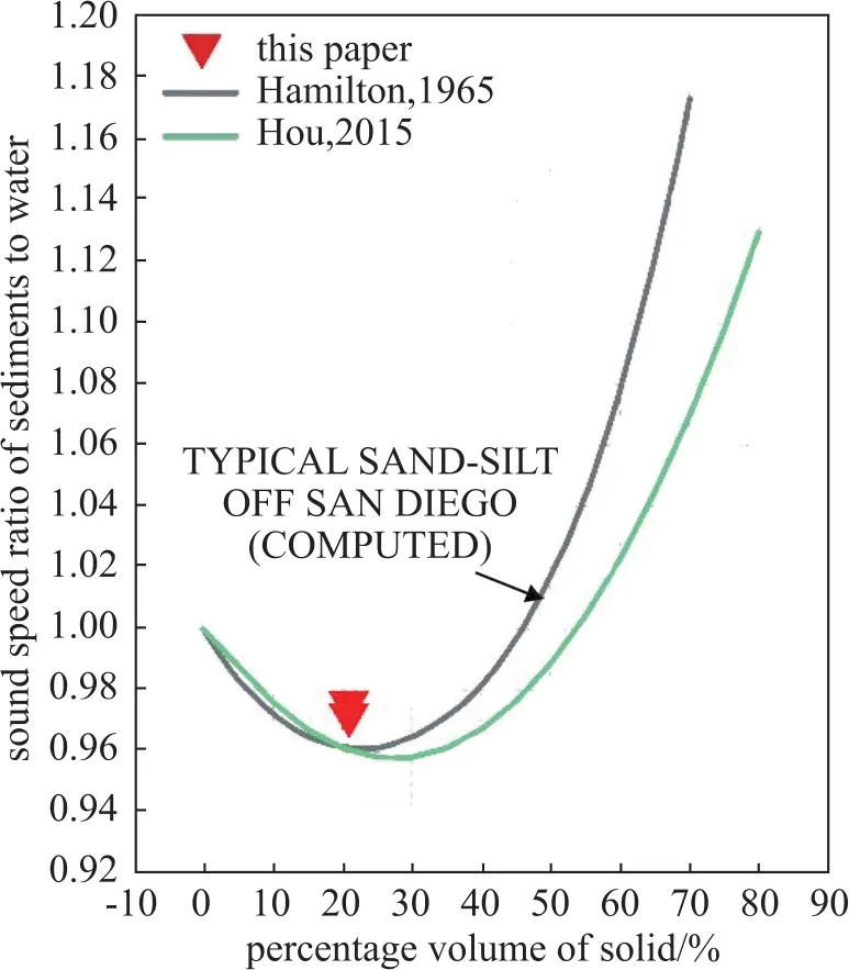
Fig.7 The relationship between sound speed ratio and percentage volume of solid from Hamilton and Hou

Hamilton explained the reason why differences in the frequency index n occur in sediments with different proportions of clay,silt,and sand.It is because all differences in sediment structures,porosities,particle sizes,contact areas between particles,and cohesive forces in sand and clay lead to differences in the attenuation measurements,which results in different frequency indices n.In addition,since it is difficult to achieve adequate accuracy of in-lab and in-situ measurements,different constants k in unit of dB·m-1·kHz-1will be expected.Hamilton determined the constant k(taking n=1)in the relationship of attenuation with the average particle sizes of most common sediments[17].The average particle size φ is expressed by φ=-log2of graindiameter ∈mm.The black curve in Fig.8 is the fitted curve by Hamilton,and the red curve is the distribution boundary of the data.The maximum value of k occurs in the average particle diameter range of φ=3.5-4.5,and the sediments mainly contain sand.When the average particle diameter φ is greater than 6,k decreases gradually to its minimum,and the content of sediments is mainly clay and silt.The average particle size of the ultrafine sediment in this study is 5.27μm measured by QL-1076 Laser Grain-Size Analyzer,and the constant k is 0.154,as indicated by a triangle in Fig.8.This result is in good agreement with the Hamilton empirical curve and is comparable to the attenuation data from in-situ measurements of South China Sea sediments with good consistency[9].Fig.8 shows that the experimental data by FITM in laboratory is reliable and the attenuation curves of saturated sediments under natural conditions given by Hamilton are applicable to the silt-clay mixed type sediments in the South China Sea.

Fig.8 The relationship between the attenuation factor k and the average particle size(For comparison,the Hamilton fitting curve[17]and the data from Wang[9]are also presented)

4.3 Comparison of the theoretical models

In this paper,the geoacoustic wave propagation models of EDFM and GS are selected to predict the sound speed and attenuation of marine sediments.The EDFM model is an extension of the Biot-Stoll model for water-saturated sediments,and the bulk modulus and shear modulus in the model are simplified to zero[14].In the GS model,the shear rigidity modulus is simplified to zero,and the compression coefficient and shear coefficient are used to express the deformation of loose saturated sediments under an external force[15].The theoretical prediction data from EDFM and GS models are compared with the measured sound speed and attenuation data in laboratory.

The input parameters of EDFM and GS models are shown in Table 2.The porosity,mass density of grains,density of fluid,grain diameter,and the depth of sediments in the grey background can be directly measured.In the EDFM model,the dynamic viscosity of pore fluid,bulk modulus of grains,and bulk modulus of fluid in the blue background are estimated from the literature[14,29-30].The permeability and tortuosity in the green background can be calculated from the measured parameters,i.e.,the porosity and grain diameter[31-33].In the GS model,the reference grain diameter,reference depth of sediments,and reference porosity in the blue background are estimated from the literature[30].The longitudinal coefficient,shear coefficient,and strain-hardening index in the purple background are obtained by fitting the dispersion relationships of sound speed and the sound attenuation at 110kHz.

Table 2 Characteristic parameters used in EDFM and GS models for sound speed and attenuation measurements.The grey background represents the directly measured parameters,the green background represents the parameters calculated from other the measured parameters,the blue background represents the estimated parameters from the literature,and the purple background represents the parameters obtained by the fitting curves of sound speed and sound attenuation at 110 kHz

For the ultrafine sediments,the sound speeds atdifferent frequencies predicted by the theoretical models was compared with the data measured by FITM in laboratory as shown in Fig.9,where the blue solid line and the red dashed line represent the sound speeds predicted by EDFM model and GS model,respectively and the triangles show the sound speed data measured by FITM in laboratory.In the 50-150 kHz frequency range,the GS model predicts lower sound speeds than the EDFM model;moreover,the two models all exhibit slightly positive dispersion characteristics.By comparing the sound speeds predicated by the models and measured in laboratory,it can be concluded that both of them show the same dispersion trend,and the sound speeds measured in laboratory are closer to those predicted by the EDFM model.This indicates that the sound speed dispersion characteristics of ultrafine sediments measured by FITM in laboratory are is reliable.

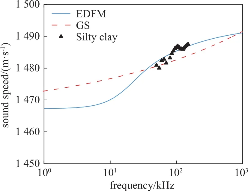
Fig.9 Comparison of the sound speeds measured in laboratory and predicted by EDFM and GS models.

For the ultrafine sediments,the sound attenuation coefficients predicated by EDFM and GS models are compared with the data measured by FITM in laboratory.As shown in Fig.10,in the 50-150 kHz frequency range,the frequency dependences of attenuation coefficient predicted by EDFM and GS models are all linear,and the trend of attenuation coefficient with frequency measured by FITM in laboratory is in good agreement with the results predicted by EDFM and GS models.By comparison it can be found that when the sound frequency is higher than 80 kHz,both EDFM and GS models can predict the sound attenuation well;when the sound frequency is lower than 80 kHz,only the GS model gives good prediction.The attenuation data predicted by EDFM and GS models show that the attenuation predicted ultrafine sediments measured by FITM in laboratory are reliable.

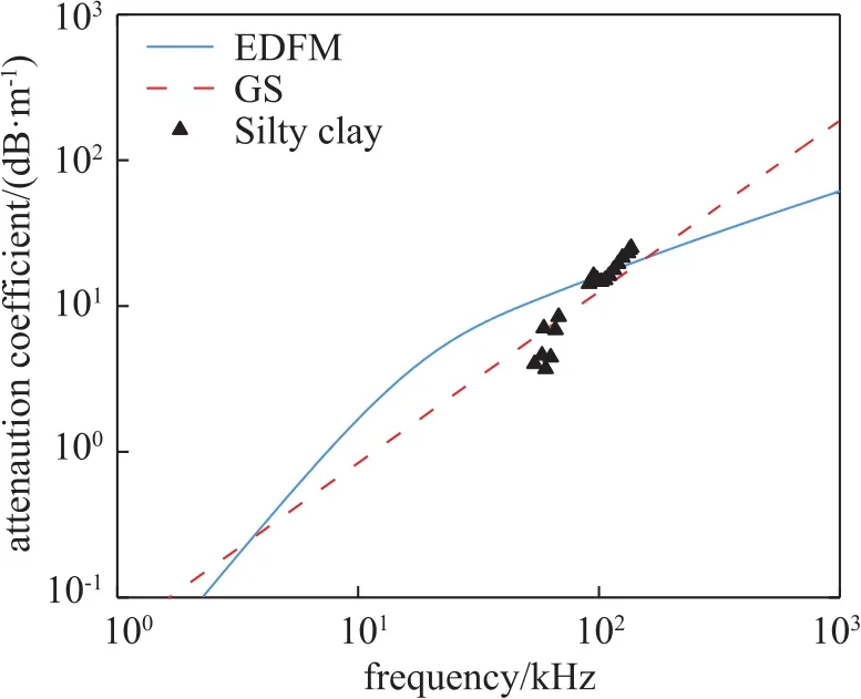
Fig.10 Comparison of the attenuation coefficients measured in the laboratory and predicted by the EDFM and GS models.

5 Conclusion

In this study,the frequency dependences of the sound speed and attenuation of ultrafine sediments are measured by using the full-immersion transducer measurement(FITM)in the 50-140 kHz frequency range.The signal generator is used to generate continuous pulse signal.Accurate data of sound speed and attenuation are obtained at multiple frequencies within the bandwidth of the transducers.The results show that for silty clay(average particle size of 5.27 μm,porosity of 79%),the sound speeds in the range of 1 480.9-1 487.5 m·s-1exhibit a weakly positive linear dispersion.The sound attenuation coefficients in the range of 4.02-25.11 dB·m-1,show a strong positive correlation with frequency.By using the Kramers-Kronig relation,the sound speeds are predicted based on a linear segment of the attenuation data measured in laboratory.The prediction results of sound speed are consistent with the measurement results in laboratory,which confirms the reliability of the experimental data.The measurement data of sound speed and attenuation in laboratory are also compared with the Hamilton data.The results show that the high porosity silty clay sediments have a low sound speed ratio and a lower attenuation coefficient.The applicability of the Hamilton sound attenuation curve to the South China Sea sediments is also verified.It demonstrates that the sound speed and attenuation of ultrafine sediments measured by FITM agree well with Hamilton empirical equation.

A comparison shows that the sound speeds measured by FITM are in good agreement with the prediction curves of the EDFM and GS models,and the prediction of EDFM model is better.The frequency dependence of attenuation measured by FITM is closer to the prediction curve of GS model than EDFM model.This provides further evidence to show the availability and reliability of FITM in the measurements of sound speed and attenuation of ultrafine sediments.