ModeIing and SimuIation for Transient ThermaI AnaIyses Using a VoItage-in-Current Latency Insertion Method

Wei Chun Chin | Boon Chun New | Nur Syazreen Ahmad | Patrick Goh

Abstract—This article presents a modeling and simulation method for transient thermal analyses of integrated circuits (ICs) using the original and voltage-in-current (VinC) latency insertion method (LIM).LIM-based algorithms are a set of fast transient simulation methods that solve electrical circuits in a leapfrog updating manner without relying on large matrix operations used in conventional Simulation Program with Integrated Circuit Emphasis(SPICE)-based methods which can significantly slow down the solution process.The conversion from the thermal to electrical model is performed first by using the analogy between heat and electrical conduction.Since electrical inductance has no thermal equivalence,a modified VinC LIM formulation is presented which removes the requirement of the insertion of fictitious inductors.Numerical examples are presented,which show that the modified VinC LIM formulation outperforms the basic LIM formulation,in terms of both stability and accuracy in the transient thermal simulation of ICs.

1.Introduction

The growth of the semiconductor industry has led to the advancement of system miniaturization technology which results in high packing densities in three-dimensional (3D) integrated circuits (ICs).In addition,higher performance has led to increased power consumption which translates to a larger amount of heat produced by these 3D ICs.Both the larger amount of heat produced per unit area and the difficulty in dissipating the heat due to the overcrowding of devices result in an increased operating temperature which can affect the performance of the IC product in a negative way[1],[2].For example,the increase of the conductor resistance by Joule heating and the distortion of the structure by thermal stress can cause the IC chips to malfunction.Thus,it is vital to understand the thermal effects in the electrical circuit in the design stages of an electronic product.

To analyze the thermal integrity of circuit designs,a verification of the thermal characteristics is often carried out.Instead of manual testing after fabrication,the software simulation at a pre-or post-layout stage is a more efficient way of analyses.Early testing and verification procedures can detect possible thermal problems in the design of IC and allow modifications to be carried out rapidly to address the issues.There are various approaches to perform thermal analyses,and a common way is by conducting a transient thermal analysis,which is just like a transient electrical analysis.But instead of the electrical behavior,the thermal behavior of the IC design versus time is analyzed.This is done by mapping the thermal model into its equivalent electrical circuit,which can then be simulated using existing electrical simulation tools.Specifically,the similarities between the laws of thermodynamics and electricity are levied to construct a thermal model of the system using electrical components,such as resistors,capacitors,and independent sources[3].The resulting equivalent circuit can then be readily simulated through available electrical simulators in the market.In this regard,the Simulation Program with Integrated Circuit Emphasis (SPICE)[4]and SPICE-based algorithms are often the preferred simulators due to their maturity and historical influence in the field of circuit simulators.However,in terms of simulation time and capacity in handling large circuits,cracks are beginning to emerge in SPICE and SPICE-based simulators.Due to their reliance on the modified nodal analysis (MNA)framework and matrix solution engines,these solvers scale poorly with the size of the circuit,and the circuits with a large number of nodes and branches can require a large amount of computational time and a large number of resources.

Attempts to solve the bottleneck in SPICE solvers have led to newer ideas and algorithms in electrical simulations,and from that,the latency insertion method (LIM) was proposed in the early 2000s[5].LIM can perform transient simulations of large networks much faster than SPICE as LIM utilizes a leapfrog analytical formulation without any matrix operation.Over the past decades,various improvements to LIM,such as block-LIM[6],partitioned LIM[7],predictor-corrector LIM[8],locally implicit LIM[9],alternating direction explicit-LIM[10],and the most recent voltage-in-current (VinC) LIM[11],have been proposed.These LIM-based algorithms have been applied to various applications including the simulations of input/output (I/O)buffers[12],[13],phase-locked loops[14],power delivery networks[15]-[18],complementary metal oxide semiconductors(CMOSs) and diodes[19]-[21],real-time power electronic systems[22],[23],stochastic[24],and transmission lines[25],[26].

In addition to these applications,LIM algorithms have been applied to perform electro-thermal analysis as well[27]-[29].However,these studies have only applied the original basic LIM algorithm,whose significant stability restriction limits the time step and hence lengthens the overall runtime of the simulation.This paper shows the application of VinC LIM for the transient thermal analysis of ICs.The VinC LIM formulation does not suffer from the stability restriction and thus is able to complete the analysis significantly faster than the basic LIM algorithm.In addition,since the equivalent thermal modeling circuit does not have inductances,a reformulation of the VinC LIM equation is presented which strips the requirement of fictitious inductances from the simulation.It is shown that the proposed formulation performs much faster and at higher accuracy than the original LIM formulation when applied to transient thermal simulations.

2.ReIated Backgrounds

In this section,the analogy between electrical and thermal systems and the fundamentals of the simulation algorithms that will be applied in the transient thermal analysis are reviewed.Discussion on the similarities between the two systems and their equivalent conversion is provided first.Then,for the simulation algorithms,the basic LIM and VinC LIM formulations are reviewed.The former is the root of the LIM-based algorithm family,while the latter is a more recent and improved LIM formulation.These two different LIM simulation algorithms are applied in this article to compare their capabilities in the transient thermal analysis from the scope of simulation stability and accuracy.

2.1.EIectricaI-ThermaI AnaIogy

Generally,heat conduction is governed by Fourier’s law which states that the rate of heat transfer ()through two points in a solid material is proportional to the temperature difference (∆T) between the two points divided by the distance between the points (∆x).It can be mathematically expressed as

wherekis the proportionality constant,also known as the thermal conductivity of the material,andAis the area normal to the direction of heat flow.On the other hand,Ohm’s law of electrical conduction states that the current (I) through an electrical conductor between two points is proportional to the voltage across the two points (∆V) divided by the resistance (R) that exists between the points.It is described by

Comparing (1) and (2),an analogy can be drawn between Fourier’s law of heat conduction and Ohm’s law of electrical conductance,where=I,∆T=∆V,and ∆x/kA=R.Table 1 summarizes the electrical-thermal analogy,where the first three rows have been explained above,and the remaining rows can be obtained by inspecting the equations governing the electrical charge and heat flux.The interested readers can be referred to [3].

Table 1: Electrical-thermal analogy

The conversion from thermal to electrical models allows the thermal analysis to be performed using electrical circuit simulators,and some examples in thermal to electrical modeling and simulations can be referred to [30] and [31].The LIM-based simulation method applied in this work will be reviewed next.

2.2.Basic LIM FormuIation

The original LIM,or basic LIM,is a circuit analysis tool built for the fast transient simulations for circuits composed of resistors (R),inductors (L),conductors (G),and capacitors (C)[5].The simulation of a circuit through LIM requires the fulfillment of LIM’s branch and node topologies shown in Figs.1 (a) and (b),respectively,whereViandVjare voltages at nodesiandj,respectively,Ii,jis the current flowing from the nodeito the nodej,Ei,jis a series voltage source,andHiis a shunt current source.

By utilizing Kirchhoff ’s law,the current and voltage in the branch and node can be solved as

Fig.1.Circuit topology required for the LIM analysis:(a) branch topology and (b) node topology.

whereLi,jandRi,jare the inductance and resistance at the branch (i,j),respectively,CiandGiare the capacitance and conductance at the nodei,respectively,and ∆tis the time step for the simulation generated from the linearization of the voltage across the inductance in the branchand the current flowing through the capacitance in the nodethrough Euler’s approximation.Thenterm in the formulation refers to the time index of the transient simulation,andMiindicates the number of branches connected to the nodei.From (3) and(4),it can be seen that the latencies,Li,jandCi,are required to be present at every branch and node in the LIM simulation.If they are not present,small fictitious elements are inserted to enable the method.In addition,in the LIM simulation,the current and voltage components are updated using a leapfrog sequence,where the currents and voltages are solved in an alternating order.This order can be seen from the indices labeled in the equations,wherenandn+1 are used for the currents,andn-1/2 andn+1/2 are used for the voltages.In this case,the current is assumed to be slightly ahead of the voltage in the simulation,but this sequence is interchangeable.

Since the LIM formulation is generated through an explicit formulation,it is only conditionally stable with a limitation on the maximum time step value.This maximum time step value can be calculated according to

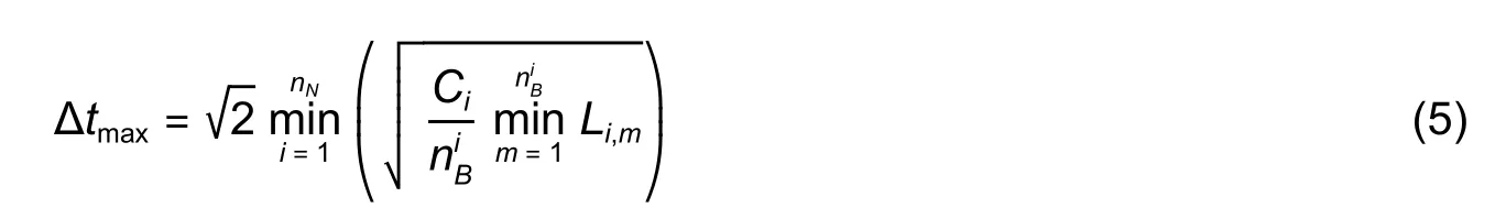
wherenNis the total number of nodes in the circuit,is the total number of branches connected to the nodei,Ciis the value of the grounded capacitance at the nodei,andLi,mis the value of the inductance in themth branch connected to the nodei[32].From (5),it can be seen that the maximum stable time step depends on the values of the capacitance and inductance in the circuit,and that smaller values will result in smaller time steps.Hence,circuits with very small latency values,especially due to the insertion of fictitious elements to enable LIM,will have severely degraded simulation performance as more iterations are required to complete the transient analysis.

2.3.VinC LIM FormuIation

VinC LIM[11]is a more recent and improved version of LIM that is derived based on an implicit formulation for enhanced stability.By writing (3) and (4) at the same time index ofn+1,the following equations are obtained

Then,substituting the voltage in (7) into (6) yields

3.ThermaI ModeIing and SimuIation Process

In this section,the procedure to carry out the transient thermal analysis is discussed in detail.First,an example thermal problem is set up,and the formation of the thermal equivalent circuit is discussed.Then,the associated LIM algorithms for the thermal simulation are presented.

3.1.ThermaI ProbIem Setup

In this article,a two-dimensional (2D) thermal problem representing an IC structure is selected,and it is based on the same thermal problem shown in [28] and [29].This example is chosen such that comparisons can be made with the results of [28] and [29].Fig.2 illustrates the thermal structure,and its corresponding dimensions,materials,heat source,and observation point.The structure has a dimension of 140 µm × 28 µm with silicon (Si) in the inner layer and silicon dioxide (SiO2) at the top and bottom layers.AB,AD,BC,and DC form the top,left,right,and bottom boundaries of the thermal problem.In these four boundaries,the DC boundary acts as an adiabatic boundary,while the other three are ambient boundaries.When heat is fed into the IC model,it can conduct freely in the model until it is finally dissipated through the AB,AD,and BC boundaries.Finally,the point E in the figure represents the measurement point for the analysis.It is to be remarked that the structure in Fig.2 is symmetric in nature,and this can be exploited to simplify the modeling and solution process with the use of a proper boundary condition.However,in this paper we will model the full structure so as to consider a general case which might be not physical symmetry.

Fig.2.2D cross section of the thermal problem.

3.2.ThermaI EquivaIent Circuit Setup

Next,the thermal problem illustrated in Fig.2 is transformed into its thermal equivalent circuit using the analogy between heat and electrical conduction.It starts with meshing the thermal structure in Fig.2 into grids with the desired dimensions.In this paper,uniform grids are formed with the dimension of 1 µm × 1 µm,similar to [28] and [29],to facilitate comparisons in the next section.This leads to the total number of 3920 thermal grid cells in the thermal problem.Fig.3 shows the meshed 2D plane of the IC structure where the red cells show the heat sources and the green cell is the measurement point.

Then,an equivalent electrical circuit is formed using the electrical-thermal analogy in Table 1,where the temperature or heat level at each grid is represented by the node voltage,and the heat flow between grids is represented by the current flow.Only horizontal and vertical connections are considered when forming the networks between grids,and the heat is restricted to flow only in these directions.Fig.4 shows the electrical circuit model of the thermal problem,where the resistors represent the thermal resistance between the grids,while the shunt capacitors represent the resulting thermal capacitance in each grid.

Fig.3.Modeling by uniform grids of the thermal problem.

The thermal resistances connecting silicon cells (Si-Si),silicon dioxide cells (SiO2-SiO2),and silicon to silicon dioxide cells (Si-SiO2) areRSi,RSiO2,andRavg,respectively.They are calculated as

where ∆xis the length of the thermal cell;Acellis the cross-sectional area of the thermal grid;kSiandkSiO2are the thermal conductivity for silicon and silicon dioxide,respectively;kavgis the equivalent thermal conductivity forRavg.The exact expression forkavgis given by 2kSikSiO2/(kSi+kSiO2),which is derived from (12).The thermal capacitanceCheatis calculated as

wherecpis the specific heat capacity of the material,ρis the volumetric density of the material at the particular thermal cell,and Vol is the volume of the thermal cell.In addition,since the AB,AD,and BC boundaries of the IC structure are ambient boundaries that allow heat convection,the thermal cells exposed to these boundaries are further connected to the ambient resistanceRambto model the heat flowing out of IC.The equation for the ambient resistance is given by

Fig.4.Electrical circuit model of the thermal problem.Heat sources are colored in red.

wherehambis the convection heat transfer coefficient andAambis the effective area of the thermal cell at the connected ambient boundary.

Table 2 summarizes the dimensions and material properties in this thermal problem.It is to be noted that since the structure is 2D,AcellandAambare equal to ∆x,while Vol is equal to (∆x)2.

Table 2: Dimensions and material properties of the thermal problem

3.3.Modified VinC LIM for Transient ThermaI AnaIysis

Once the equivalent circuit of the IC model has been constructed,suitable electrical simulation algorithms can be applied to run the transient thermal analysis.In this article,the basic LIM and VinC LIM algorithms are applied.For the basic LIM simulation,an inductance in each branch is necessary for the branch updating equation to be performed correctly.Since the thermal model does not have equivalence for electrical inductances,a small fictitious inductance is inserted in series to the thermal resistance in each branch.The choice and effect of the value of this inductance will be investigated in the next section.

For the VinC LIM simulation,a reformulation is performed which removes the need of the inductances from the simulation.First,the current expressed by (6) is rewritten without theLi,jterms to yield

Then,the voltage shown by (7) is substituted into this new current equation to yield

The VinC LIM simulation can then be performed using the modified equation shown in (17) in place of (9).Note that noLi,jterms exist in the formulation and thus no fictitious inductances need to be inserted.

4.ResuIts and Discussion

In this section,the thermal circuit is simulated using the basic LIM and modified VinC LIM formulations.Results are presented,which compare the performance of the algorithms in terms of stability and accuracy,with consideration on the time step of the simulation.First the circuit in Fig.4 is simulated using both algorithms and Fig.5 shows the overall thermal behavior of the IC model at the end of the simulation.The thermal distribution map shows the conduction of heat from the source to the entire 2D IC model.It can be seen that the heating effect at the upper part is averagely lower than the bottom part due to the ambient boundaries that allow heat dissipate to the surrounding,compared with the adiabatic boundary at the bottom which results in more heat stored in the lower part of IC.

Next,the temperature at the point E (see Fig.3)of the IC structure is plotted in Fig.6.Multiple simulations are carried out with different time steps,starting from 30 ns,which is the calculated maximum stable time step through (5) when the inserted fictitious inductance is 1 nH.Note that for the VinC LIM simulations,no fictitious inductances are inserted.It can be seen that the simulation using basic LIM is stable only for the time step of 30 ns,and any simulations using the time step which is larger than 30 ns are unstable,while the VinC LIM formulation remains stable for all time steps.

Fig.5.Temperature distribution of the simulated IC model in °C.

Fig.6.Basic LIM and VinC LIM simulations with different time steps.The 1-nH fictitious inductance is inserted in basic LIM and no fictitious inductances are required in VinC LIM.

Since basic LIM is only conditionally stable as given by (5),in order to run the simulation with larger time steps,the value of the fictitious inductance must be increased,however,which will have an adverse effect on the accuracy of the simulation.Fig.7 (a)shows the simulation results by using a larger fictitious inductance in basic LIM,in order to relax the simulation time step.As a comparison,Fig.7 (b)shows the simulations using the same time steps in VinC LIM without any fictitious inductance.It can be seen that the simulations using basic LIM show significantly larger degradation in accuracy with larger time steps,compared with VinC LIM.Table 3 shows the root mean square (RMS) errors of the simulations as compared with the simulation at the time step of 30 ns.It can be seen that the RMS errors are significantly lower in the VinC LIM simulations for the same time steps.This shows the superiority of the presented modified VinC LIM formulation which does not require any fictitious inductance.

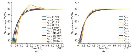
Fig.7.Simulated waveforms at different time steps from (a) basic LIM (values of fictitious inductances are written in parentheses) and (b) VinC LIM (no fictitious inductances are required in VinC LIM).

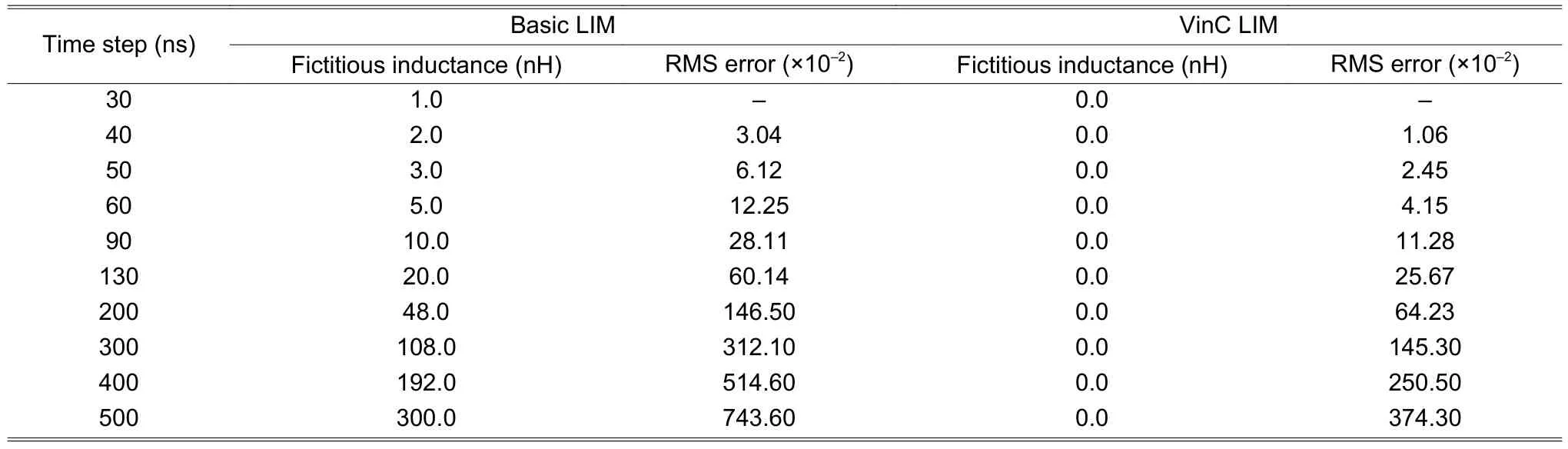
Table 3: RMS errors in basic LIM and VinC LIM simulations at different time steps

In addition,Table 4 compares the simulation runtime of the proposed VinC LIM algorithm and SmartSpiceTM,a modern simulator from Silvaco,for the same thermal model but with varying thermal cell lengths of 1.00 µm,0.50 µm,and 0.25 µm at the time step of 30 ns.The results show that the proposed framework is much faster at solving the same model and the speedup ratio increases with the size of the circuit.

Table 4: Runtime and speedup comparison between SmartSpice and VinC LIM for the simulation time step of 30 ns

To draw a comparison with previous work,the data from the same simulations in [28] and [29] are referred to.For a 1-µm mesh model,the results in these papers showed that basic LIM,at its minimal time step of 28.7 ns,obtains a similar level of accuracy compared with the commercial software COMSOL Multiphysics and the Gauss-Seidel (GS) method,while being 11.5 folds and 107.8 folds faster than them,respectively.As a comparison,the results from the modified VinC LIM simulation presented in this paper at the time step of 500 ns would be approximately 17.4 folds faster than that from the basic LIM simulation at 28.7 ns,and hence approximately 200 folds and 1875 folds faster than those from COMSOL Multiphysics and GS,respectively.All these results show the potential of the VinC LIM formulation in electro-thermal simulations.

5.ConcIusion

In this work,the modeling and simulation method for transient thermal analyses is presented using LIM.Using the electrical-thermal analogy,an electrical equivalent circuit is formed to model the heat conduction problem.Since there is no equivalence for the electrical inductance in heat conduction,a modified formulation is presented for the VinC LIM,which does not require the insertion of fictitious inductances.Results show that the proposed modified formulation is much better in terms of stability and accuracy compared with the basic LIM formulation.Future work will focus on the complete 3D modeling of IC systems towards providing electrothermal co-simulation solutions.

DiscIosures

The authors declare no conflicts of interest.