An Improved Hyperplane Assisted Multiobjective Optimization for Distributed Hybrid Flow Shop Scheduling Problem in Glass Manufacturing Systems

Yadian Geng and Junqing Li,2,★

1College of Computer Science,Liaocheng University,Liaocheng,252059,China

2School of Information Science and Engineering,Shandong Normal University,Jinan,25014,China

ABSTRACT To solve the distributed hybrid flow shop scheduling problem (DHFS) in raw glass manufacturing systems, we investigated an improved hyperplane assisted evolutionary algorithm(IhpaEA).Two objectives are simultaneously considered, namely, the maximum completion time and the total energy consumptions.Firstly, each solution is encoded by a three-dimensional vector, i.e., factory assignment, scheduling, and machine assignment.Subsequently,an efficient initialization strategy embeds two heuristics are developed,which can increase the diversity of the population.Then,to improve the global search abilities,a Pareto-based crossover operator is designed to take more advantage of non-dominated solutions.Furthermore,a local search heuristic based on three parts encoding is embedded to enhance the searching performance.To enhance the local search abilities,the cooperation of the search operator is designed to obtain better non-dominated solutions.Finally,the experimental results demonstrate that the proposed algorithm is more efficient than the other three state-of-the-art algorithms.The results show that the Pareto optimal solution set obtained by the improved algorithm is superior to that of the traditional multiobjective algorithm in terms of diversity and convergence of the solution.

KEYWORDS Distributed hybrid flow shop;energy consumption;hyperplane-assisted multi-objective algorithm;glass manufacturing system

1 Introduction

The hybrid flow shop scheduling problem (HFS) has been investigated and employed in lots of realistic industrial applications[1],such as glass-making systems[1–3]and steelmaking systems[4].In the classical HFS process, there are several jobs, machines, and stages.A certain number of parallel machines are in each stage,where each arriving job should choose exactly one available machine.And each job follows the same processing route with machine selection flexibility.Therefore,compared with the classical flow shop scheduling problem,in HFS,an additional task is selected to suit machines for each operation,which has been proven to be an NP-hard problem[1].

With the development of industries, more and more researches have focused on distributed scheduling problem, including the distributed flow shop scheduling problem (DFSSP) [5], as well as distributed hybrid flow shop scheduling problem (DHFS) [6].However, there is less literature for DHFS, compared with the works in solving flow shop or distributed flow shop.Pan et al.[7] studied a distributed flowshop group scheduling problem (DFGSP), where the families are considered in manufacturing cells.Huang et al.[8] proposed three constructive heuristics and an effective discrete artificial bee colony(ABC)algorithm to solve the distributed permutation flowshop scheduling problem.Meng et al.[9]introduced the lot-streaming and carryover sequence-dependent setup time in the distributed permutation flowshop scheduling problem(DPFSP)with non-identical factories.Ying et al.[10] developed a hybrid algorithm with three versions of iterated greedy (IG)algorithm in order to minimize the makespan of the DHFS.Hao et al.[11] considered a DHFS with a brain storm optimization (BSO) algorithm, where the makespan is minimized.Cai et al.[12]proposed a new shuffled frog-leaping algorithm(SFLA)with memeplex quality(MQSFLA),which was used to minimize total tardiness and makespan simultaneously.Shao et al.[13]proposed a multineighborhood IG algorithm so as to solve the problem.Li et al.[14] investigated an improved IG algorithm to solve the DPFSP with both robotic transportation and order constraints.Jiang et al.[15]studied the energy-aware DHFS with multiprocessor tasks with considering total energy consumption and makespan.Niu et al.[16]developed an improved NSGA-II algorithm to solve an energy-efficient distributed assembly blocking flow shop problem.Qin et al.[17] utilized a realistic DHFS where a novel integrated production and distribution scheduling problem is focused.

In realistic industry system,including the glass manufacturing system,the improvement of glass raw materials processing has been studied by many researches[18–20],and therefore,the scheduling efficiency has become increasingly important[21].Na et al.[22]addressed the glass optimization problems by using heuristic methods.Lozano et al.[23]proposed a two-phase heuristic that combines exact methods and searching heuristics.Wang et al.[24] proposed two heuristics based on decomposition idea to minimize total electricity cost and makespan.Wang et al.[25] formulated a mixed integer programming (MIP) for the problem.Typically, a highly energy-consuming stage (i.e., depreciation of machinery)exits in glass making process,which takes up a large part of the production cost.As a result,considering energy consumption in glass manufacturing system is practical as well as necessary.

Recently, multiobjective optimization algorithms have been applied and considered in many domains[26–31].Shahvari et al.[32]considered a tabu search(TS)algorithm to minimize two different objectives.Zhang et al.[33]proposed a novel multiobjective multifactorial immune algorithm with a novel information transfer method to deal with multiobjective multitask optimization problems.Wang et al.[34]improved the overall efficiency of optimizing multiple tasks simultaneously by reusing the learned knowledge.Li et al.[35]solved flow shop scheduling problems with a novel multiobjective local search framework-based decomposition.Li et al.[36]developed a knowledge-based adaptive reference points multi-objective algorithm(KMOEA)to solve a DHFS with variable speed constraints.Du et al.[37]proposed a hybrid multi-objective optimization algorithm based on an estimation of distribution algorithm (EDA) and deep Q-network to solve a flexible job shop scheduling problem (FJSP) with time-of-use electricity price constraint.Mou et al.[38] developed an effective hybrid collaborative algorithm for energy-efficient distributed permutation flow-shop inverse scheduling.Li et al.[39]proposed an improved artificial immune system(IAIS)algorithm to solve a special case of the FJSP in flexible manufacturing systems.However,less literature investigated the multi-objective optimization in glass manufacturing systems.

Therefore, to solve DHFS in glass manufacturing systems,we propose an improved hyperplane assisted evolutionary algorithm(IhpaEA).The main contributions of this study are as follows:(1)each solution is represented with a three-dimensional vector, including the factory assignment, machine assignment,and operation scheduling;(2)an efficient initialization strategy is developed to increase the diversity of the population(3)an improved crossover operator is designed to enhance the global search abilities of the proposed algorithm;and(4)a cooperative search method is designed to enhance the local search abilities of the proposed algorithm deeply.

The structure of the rest paper is as follows.The problem descriptions are given in Section 2.Next,the developed IhpaEA framework is presented in Section 3.Then, the detailed components of the imposed algorithm are discussed in Section 4.Section 5 illustrates the experimental results to show the advantages of the algorithm.Finally, the last section shows the conclusion and future research directions.

2 Problem Description

The DHFS addressed in this study can be described as follows.There arenindependent jobs to be assigned toffactories.Each factory consists of a series ofπiproduction stages(or processing centers)where there arekparallel machines in each stage.Moreover,each job can be completed in any factory with the same sequence.Each operation can be processed on any selected machine at the corresponding stage.

2.1 Problem Formulation

1)Assumptions:

· Each job should be released at time zero and be operated from the first stage to the next stage;

· All machines are available at time zero and remain continuously available over the entire production horizon;

· A job can be processed on exactly one machine at a time, and a machine can process exactly one job at a time;

· At each stage,one job can select one suitable machine from the parallel machine;

· There is unlimited buffer between stages;

· All machines belonging to the same stage have similar processing abilities.

2)Notations and variables:

Indices:

iIndex of the machines.

jIndex of the jobs.

fIndex of the factories.

kIndex of the stages

Parameters:

nNumber of jobs.

mNumber of machines.

wNumber of stages.

hNumber of factories.

mkNumber of machines ink thstage,fork=1,2,...,w.

JjJobj,fori=1,2,...,n.

MiMachinei,fori=1,2,...m.

Oijithoperation of jobj.

niNumber of jobs that are processed onMi.i=1,2,...m.

Jirrthjob that is processed onMi.i= 1, 2,...m,r= 1, 2,...,m.

Variables:

SStarting time ofOij.i=1,2,...,m,j=1,2,...,n.

CmaxMakespan,i.e.,the maximum completion time.

PMfkiMachine power ofMiin stagekof factoryf,k= 1,2,...,w,i= 1,2,...,m,f=1,2,...,h.

TMfkiMachine working time ofMiin stagekof factoryf,k= 1,2,...,w,i= 1,2,...,m,f=1,2,...,h.

TECTotal energy consumption.

Decision Variables:

xjfA binary decision variable,which equals to 1 when jobJjis assigned to factoryfand otherwise equals to 0.

zijA binary decision variable, which equals to 1 when jobJjis processed onMiand otherwise equals to 0.

3)Objective functions:

The makespan (Cmax) and TEC are considered as two objectives.The first objective is to minimize makespan whereCmax=The second objective is to minimizeTECwherei.e., the total energy consumptions during the processing time for all machines.

2.2 Realistic Problem Example

A detailed illustration of the considered realistic DHFS is presented in a glass manufacturing casting system in Fig.1.A specified quantity of molten glass can be provided by three processing stations.Many beam carriers(BCs)are used to transport those pouring molten glass.Each job or BC is transported to an available factory.The molten glass transported by BC will be operated through at least two stages in each factory:1) glass forming; and 2) heat treatment stages.The processing operations are the same in all the factories for each BC.After processing in the designated factory,BC will be moved to the next stage,in which one machine will be selected for continuous casting procedure.The specified amount of charging shall be handled for each assigned machine.Fig.1 presents that the complete working flows in the basic glass manufacturing casting system which can be considered as a typical DHFS with several stages in the last part.Moreover,the realistic processing systems should consider the deteriorating job constraint[33,34].

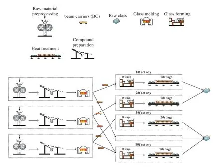
Figure 1:Realistic DHFS problem in a glass manufacturing system

A common production flow is shared by different glass manufacturing systems, i.e., raw glass should experience preprocessing, melting, and forming processes in sequence, as shown in Fig.2.Specific processing requirements or features are in individual manufacturing systems with the considering that various types of glass are provided by different manufacturers.The detailed processing characteristics of this study are as below:

(1) Raw material preprocessing:Crush large raw materials(soda,quartz sand,feldspar,limestone,etc.)to dry raw materials which are wet,and then remove iron from raw materials to ensure glass quality.

(2) Compound preparation.

(3) Glass melting:In order to make the glass raw materials meet the forming requirements of uniform,bubble free and molten liquid glass,the glass raw materials need to be placed in the pool kiln or crucible kiln and heated at high temperature(1500–1600 degrees).

(4) Glass forming:Liquid glass is processed into the required shape of the specific products.

(5) Heat treatment:Through annealing,quenching and other processes to change the structural state of glass.

3 Methodology

In this section, the proposed IhpaEA algorithm is presented to solve the considered DHFS problem.The first part describes the main framework of the proposed IhpaEA.Then the encoding,decoding,initialization,crossover,and other problem-specific heuristics are presented,respectively.

3.1 Framework of the Proposed IhpaEA

The main framework of the proposed IhpaEA algorithm is an enhanced inverted GA (genetic algorithm) indicator based hpaEA [40].In IhpaEA, the main components, including the uniform reference point,mating selection and the environmental selection functions are directly included from hpaEA.The prominent solutions are retained by the environment selection strategy of hyperplane assisted evolutionary algorithm.Besides, it uses two criteria to select the size of population and the non-dominated solutions.

Algorithm 1 represents the framework of IhpaEA, where the first step is to initialize four parameters (1) an initial population P (line 1); (2) vectors V (line 2); (3) the number of prominent solutions (line 3) and (4) the evaluation functions (line 4); and the loop of IhpaEA (lines 5–12).Each generation performs three steps in the algorithm:(1)mating selection;(2)offspring population generation, and (3) environmental selection.The mating selection tries to assign more evolutionary results to the prominent solutions, and select better solutions.The set {1,2,...,K} represents the prominent solutions whereKstanding for the number of prominent solutions, which will be firstly chosen and located in the front of the population for environmental selection.The indexes of the solutions selected for mating are denoted as tan arrayI.N-Ksolutions are first randomly selected(line 6)in the current populations to form the mating pool.Although some of the prominent solutions have been selected randomly in the former step, and allKpromising solutions are chosen (line 7).Finally,rearrange all the elements in the arrayI(line 7).Next,an Improve Similar Job Order Crossover I (ISJOXI) is used by the proposed IhpaEA to produce the offspring population (line 8), which is different from the studies[40].Besides,populationQ(line 12)performs the environmental selection strategy.

3.2 Representation and Encoding

Each solution is represented by a three-dimensional vector as follows.

The first dimensional vector is called scheduling vector, and the length of it equals to the total number of operationsΠ= {π1,π2,..,πn}.Each job number represents an element of the scheduling vectorπi,and the order of arrangement is the sequencing order.

The name of the second dimensional vector is called the machine assignment vectorδ={δ1,δ2,...,δk},elementδiof the vectors is represented by a machine number which tells the machine assigned to the corresponding job.

The third dimensional vector is named as the factory assignment vector,and the length of factory assignment vector equals to the total number of jobsφ= {φ1,φ2,...,φn}, Each element of the factory assignment vectorφiis represented by a factory number, which tells the factory assigned to the corresponding job.

Fig.3a gives a solution representation example, where there are five jobs.The total number of stages for each job is 2.The factory assignment vector tells the factory number for each job,the routing vector reports the machine number.Then, the scheduling vector represents the scheduling sequence for each job.

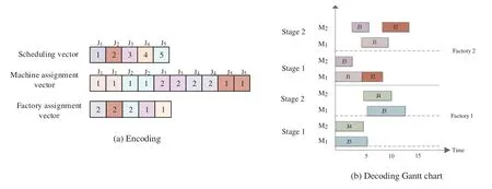
Figure 3:Solution representation

3.3 Decoding Heuristic

Fig.3b shows the Gantt chart.The detailed decoding introduces are described as follows:

Step 1:The assigned jobs are scheduled based on the sequence in the scheduling vector which is the first stage of each factory.

Step 2:After determining the factory, each job should select a suitable machine following the earliest available time rule.

Step 3:For the other stages,each job is scheduled as soon as possible after completing its previous operations.The first available suitable machine is also selected.

3.4 Initialization

To solve the considered problem, a solution is encoded with two dispatching rules.The longest processing time at the first stage(LPTF)rule,and the shortest processing time at the first stage(SPTF)rule.Based on the non-increasing total processing times,LPTF generates a permutation.Meanwhile,based on the non-decreasing total processing times,SPTF produces a permutation by sorting the jobs.

To produce an effect initial population,the following technique is used.Suppose the population size isN,the detailed steps are given as follows:

(1) The firstN-2 individuals are generated by a random way.For the factory assignment vector,each job is assigned to a random selected factory.For the scheduling vector,all the jobs are sequenced in a random order.

(2) One individual is generated by LPTF.First, all the jobs’processing time are calculated in each stage.Then,every job in every stage has a processing time and the summation of these time is called total processing time.Finally,the individual is generated by permuting the total processing time in non-increasing order.

(3) SPTF generates the last individual.The first two steps are the same with LPTF.However,the third step is to permute the processing time in a non-decreasing order.

3.5 Crossover

Based on the encoding representation, we proposed a novel crossover heuristic including two parts.

(1) PTL crossover

The first type of crossover is PTL,which can be described as follows:

Step 1:Randomly select two different elements from the first parent.

Step 2:Copy the block of jobs which are cut by the two points from the first parent.And then move the block to the rightmost or leftmost part of the offspring.

Step 3:Place the empty elements of jobs which are remaining from the second parent.

The process of PTL for generating offspring is depicted in Fig.4.Table 1 provided an example which can figure out the way element are updated.

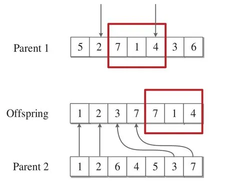
Figure 4:PTL crossover operator

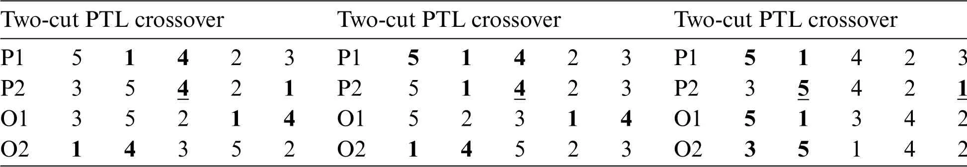
Table 1:An example of PTL crossover operator

(2) ISJOXI crossover

The second type of crossover operator is Improve Similar Job Order Crossover I or ISJOXI,with which the building blocks of jobs are directly copied to the offspring.In Fig.5a,a point is randomly selected and the elements before this cut point is copied to the offspring directly, shown in Fig.5b.Furthermore, in order to maintain feasibility of the job sequence, the ISJOXI crossover operator copies the missing elements of each offspring which are in the relative order of the other parents,shown in Fig.5c.Lastly, other elements which are not assigned are obtained by performing single point crossover operator onP1andP2which is chose a crossover point randomly between elements 2 and 3.In this example,r1andr2are selected as crossover points.Then,the elements betweenr1andr2are copied fromP1,and the elements afterr2are copied fromP2.However,since J5 is absent,and J1 appears twice,J1 in offspring1 should be substituted with J5.As a result,offspring1 will be(1,2,5,7,4,3,6)and offspring 2 is generated in the same way,which is(5,2,4,1,7,3,6),as shown in Fig.6.

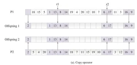
Figure 5:(Continued)

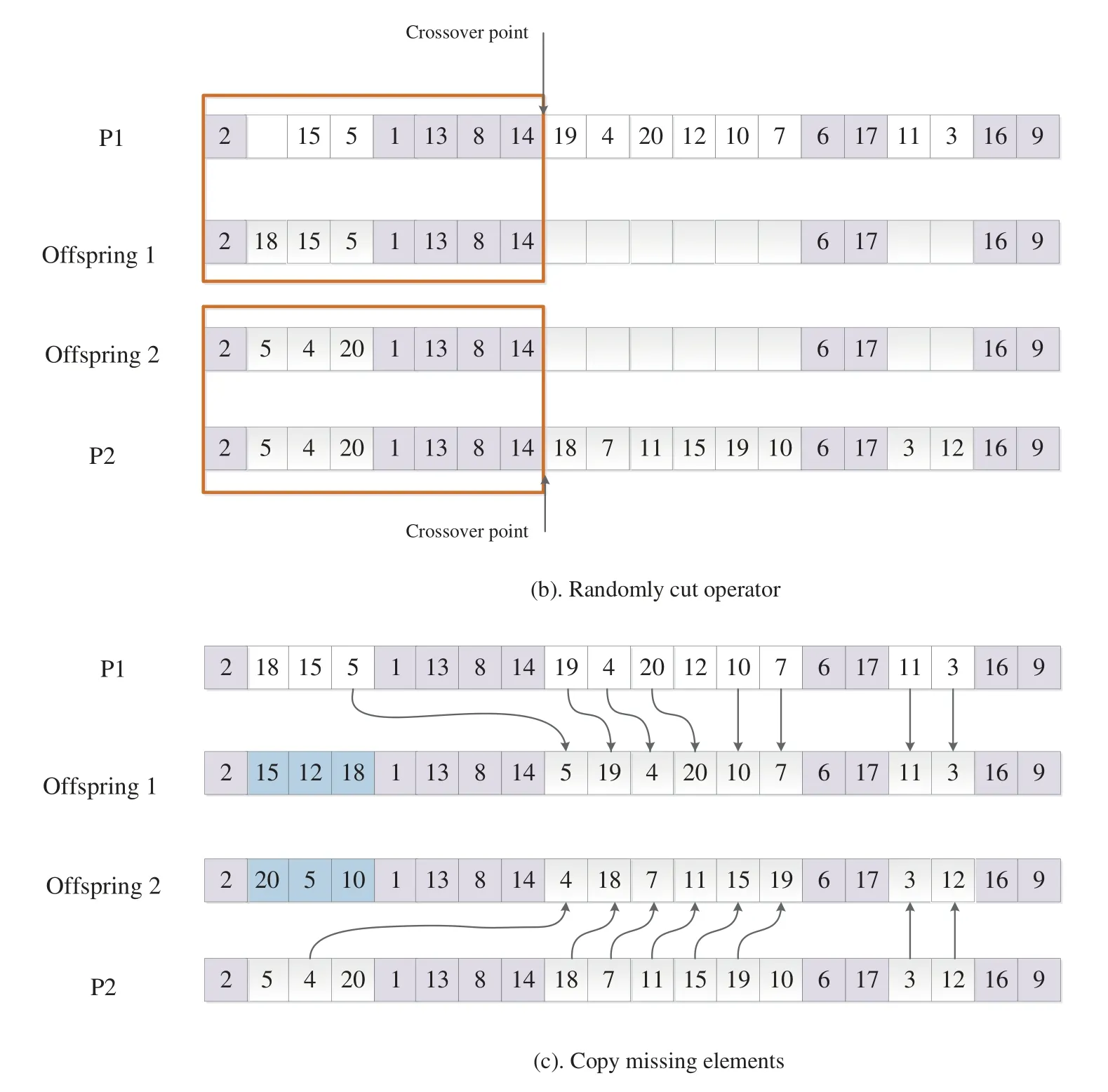
Figure 5:Process of performing ISJOXI

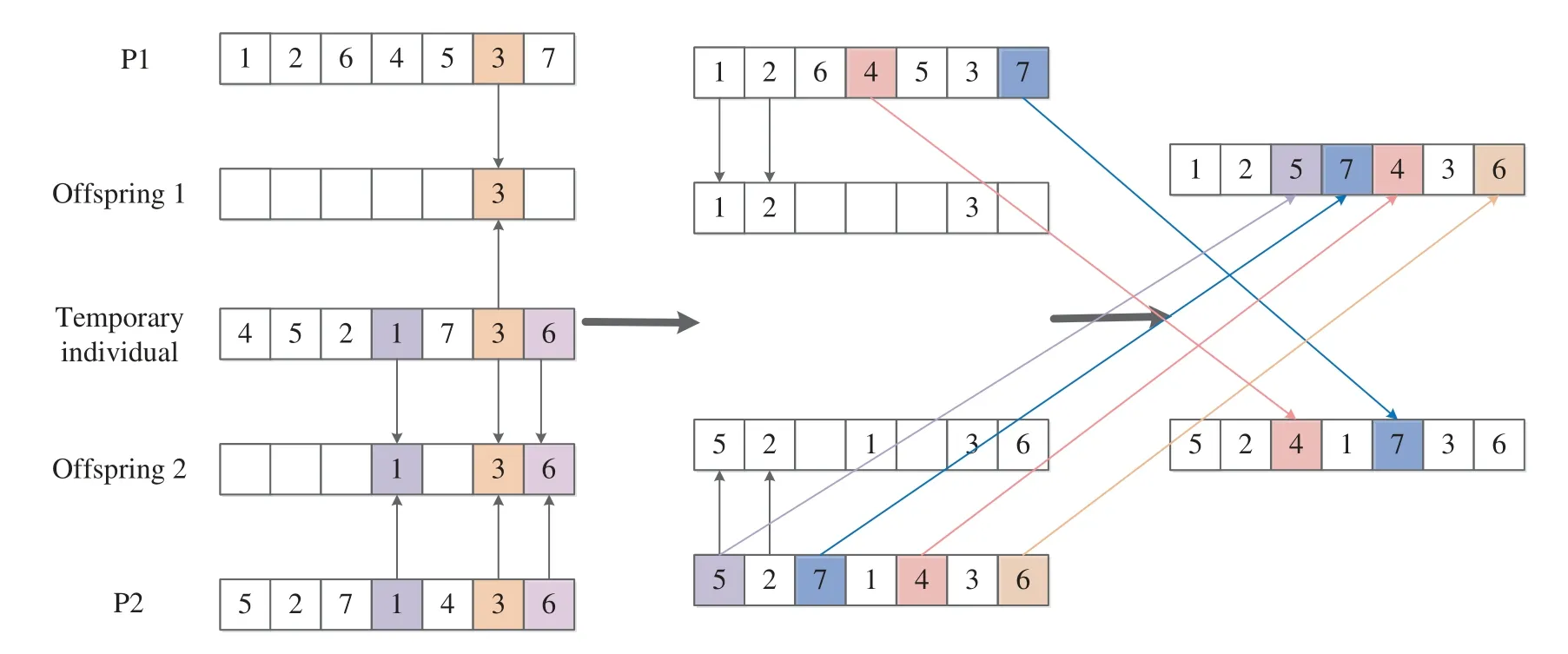
Figure 6:ISJOXI

The main steps of ISJOXI crossover are described in Algorithm 2.

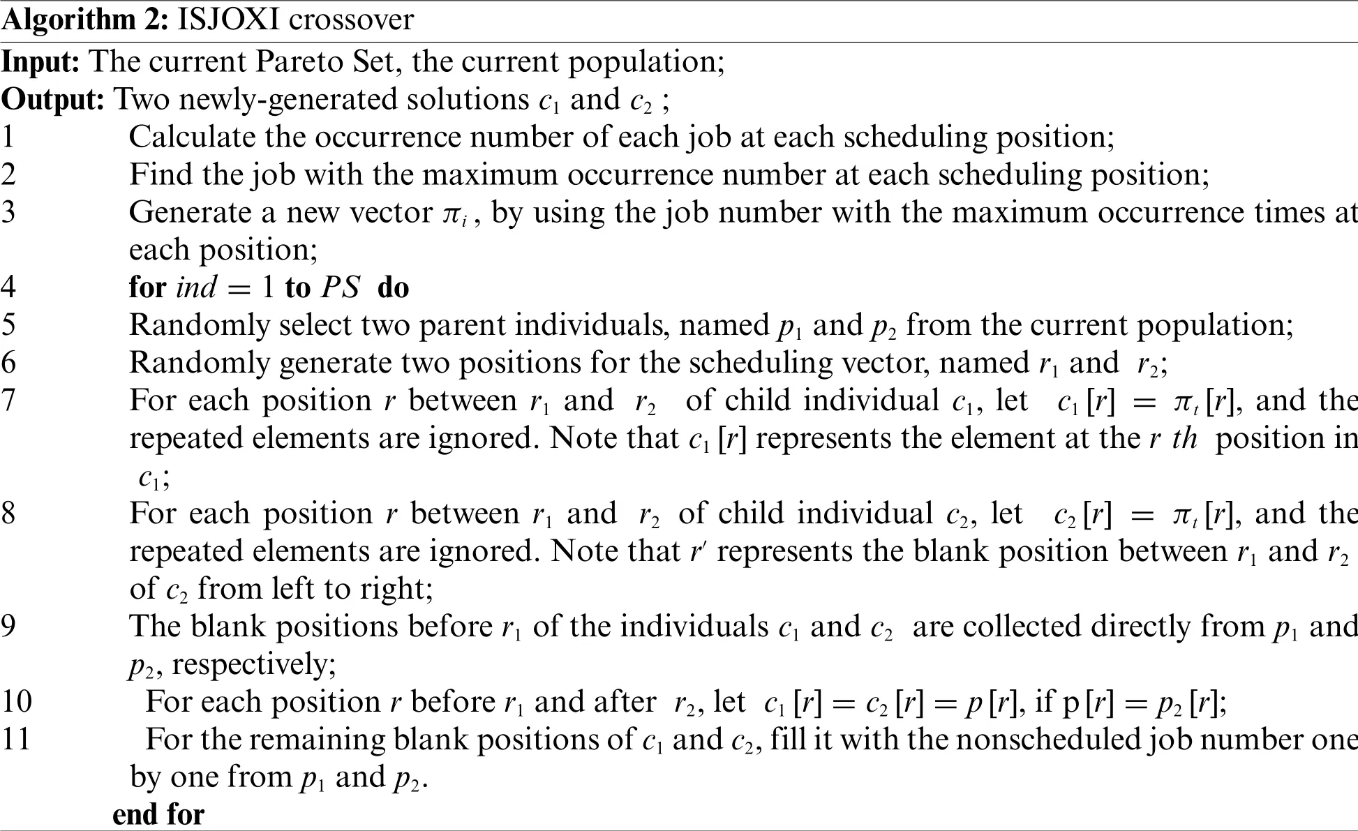
Algorithm 2:ISJOXI crossover Input:The current Pareto Set,the current population;Output:Two newly-generated solutions c1 and c2;1 Calculate the occurrence number of each job at each scheduling position;2 Find the job with the maximum occurrence number at each scheduling position;3 Generate a new vector πi,by using the job number with the maximum occurrence times at each position;4 for ind =1 to PS do 5 Randomly select two parent individuals,named p1 and p2 from the current population;6 Randomly generate two positions for the scheduling vector,named r1 and r2;7 For each position r between r1 and r2 of child individual c1, let c1[r] = πt[r], and the repeated elements are ignored.Note that c1[r]represents the element at the r th position in c1;8 For each position r between r1 and r2 of child individual c2, let c2[r] = πt[r], and the repeated elements are ignored.Note that r′represents the blank position between r1 and r2 of c2 from left to right;9 The blank positions before r1 of the individuals c1 and c2 are collected directly from p1 and p2,respectively;10 For each position r before r1 and after r2,let c1[r]=c2[r]=p[r],if p[r]=p2[r];11 For the remaining blank positions of c1 and c2,fill it with the nonscheduled job number one by one from p1 and p2.end for

3.6 Mutation

SupposeFcis the factory with the maximum makespan,andFeis the factory with the maximumTEC.The mutation method for the DHFS problem is described as follows:

(1)Mutation for the factory assignment

FAcs:Select two jobsJ1andJ2randomly,whereJ1fromFcandJ2from a different factory,then swap the two positions of them.

FAes:Select two jobsJ1andJ2randomly,whereJ1fromFeandJ2from a different factory,then swap two positions of them.

FAci:Randomly insert a job which is removed fromFcinto a location in a randomly selected factory.

FAei:Randomly insert a job which is removed fromFeinto a location in a randomly selected factory.

(2)Mutation for the scheduling vector

JScs:Randomly choose two different jobs fromFcand then swap them.

JSes:Randomly choose two different jobs fromFeand then swap them.

JSci:Insert a job which is randomly selected into a random location inFc.

JSei:Insert a job which is randomly selected into a random location inFe.

(3)Mutation for the machine vector

The procedure of the mutation operator is as follows.Firstly,a positionr1is randomly selected in the machine vector.Then for the element inr1,select a different machine.

3.7 Local Search

The following multi-objective cooperation local search operator is embedded to achieve good diversity and convergence.First, in each generation, the maximum completion time of solutionais denoted asand the TEC of each solutionais denoted as(TEC(a)-TECmin)/(TECmax-TECmin) whereTECmin,TECmax,,represent the minimumTEC, maximumTEC, minimum makespan and maximum makespan of the solutions in current population.

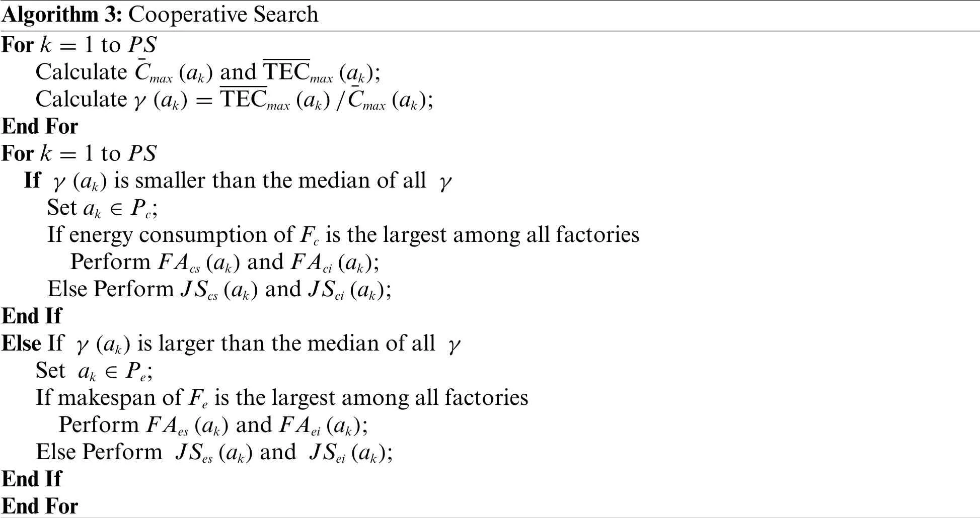
Algorithm 3:Cooperative Search For k=1 to PS Calculate ¯Cmax(ak)and TECmax(ak);Calculate γ (ak)=TECmax(ak)/¯Cmax(ak);End For For k=1 to PS If γ (ak)is smaller than the median of all γ Set ak ∈Pc;If energy consumption of Fc is the largest among all factories Perform FAcs(ak)and FAci(ak);Else Perform JScs(ak)and JSci(ak);End If Else If γ (ak)is larger than the median of all γ Set ak ∈Pe;If makespan of Fe is the largest among all factories Perform FAes(ak)and FAei(ak);Else Perform JSes(ak)and JSei(ak);End If End For

An example is provided in Table 2,where the objective values of a population with four solutions are listed,including theCmaxandTECof each solution.According to theγ,these solutions are divided intoPcandPe.From Table 2,a1anda3are put intoPc,a2anda4are put intoPe.For solutiona1,Fe=1 and the makespan ofFeis medium among all factories.As a result,it performsJSesandJSeiin turn for solutiona1.For solutiona2,Fc= 3 and theTECofFcis the largest among all factories.Thus,it performsFAcsandFAciin turn for solutiona2.

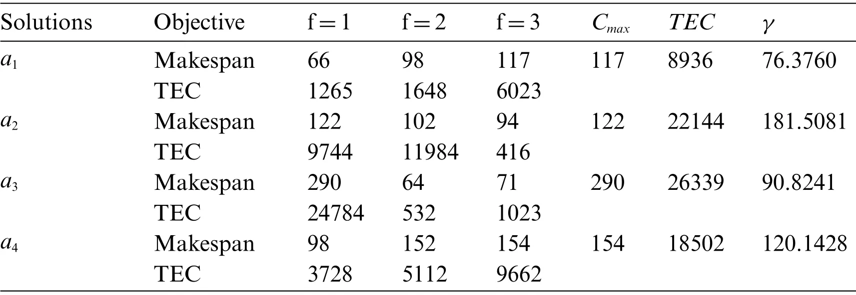
Table 2:Example for collaborative search

4 Experimental Results

The computational experiments to test the performance of IhpaEA algorithm is discussed in this section.The improved algorithm was implemented in the PlatEMO v3.0 on an Intel Core i7 3.4-GHz PC with 16 GB of memory.To test the performance of IhpaEA algorithm, 20 different scales of instances are generated according to the realistic flow shop.

All the compared algorithms are used to solving the considered problem,including the encoding,and decoding method, and the initialization procedure.The parameters are set according to their literatures.For each instance,the stop condition is set to 3000 iterations.

30 independent runs are used to test the performance of the proposed algorithm, the results of non-dominated solutions found by all the compared algorithms were collected for performance comparisons.The relative percentage increase (RPI) is used for the ANOVA comparison, which is formulated as follows:

whereCbrepresents the best solution that has been calculated by all the compared algorithms andCcis the best solution to the tested algorithm.

4.1 Experiment Parameters

20 large-scale test instances of DHFS problem are randomly generated to solve the DHFS problem and test the validity of the hpaEA algorithm based on the actual production data.For example,instance 1 can be denoted with 20 jobs, 2 stages, as well as 3 parallel machines in the first stages as well as 5 parallel machines in the second stages wherein the index of jobs are{20,30,50,80,100},the parameter of machines are{2,3,4,5},the parameter of stages are{2,3,5,10},and the parameter of factories are{2,3,4,5,6},respectively.The four algorithms ran 30 times.

4.2 Efficiency of the Initialization Heuristic

Two types of IhpaEA algorithms are coded to test the initialization heuristic discussed in Section 3.4:a random initialization heuristic named IhpaEA-NI,and IhpaEA with all components.All other components of the two comparison algorithms are the same.

Table 3 reports the comparison results between IhpaEA-NI and IhpaEA.Instance numbers are given in the first column,the HV results collected from the two compared algorithms are listed in the following two columns,respectively.The last two columns illustrate the IGD values by IhpaEA-NI and IhpaEA,respectively.

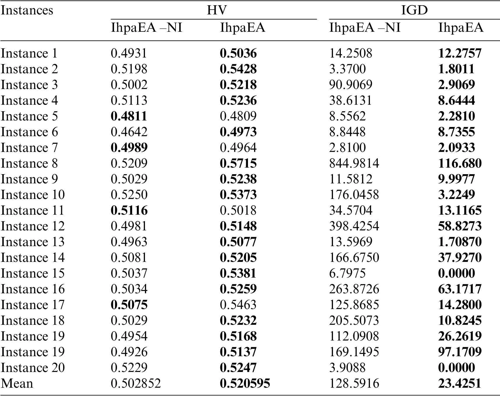
Table 3:Comparisons between IhpaEA–NI and IhpaEA

It can be concluded from the comparison results that:(1) IhpaEA algorithm obtains 16 better results by considering the HV values of the IhpaEA-NI algorithm,and the slightly worse results for the other two instances; (2) for the IGD values, IhpaEA obtains 20 better results out of the given 20 different scale instances; and (3) from the average performance in HV and IGD given in the last line and the ANOVA results from Fig.7a,it can be seen that IhpaEA is significantly better than the IhpaEA-NI algorithm,which verify the efficiency of the proposed initialization heuristic.

4.3 Efficiency of the Crossover Operator

In order to test the performance of the crossover operators discussed in Section 3.5,two different types of IhpaEA algorithms are coded, i.e., the IhpaEA-NC algorithm with the classical two-point crossover,and the IhpaEA algorithm with all the two crossover operators.

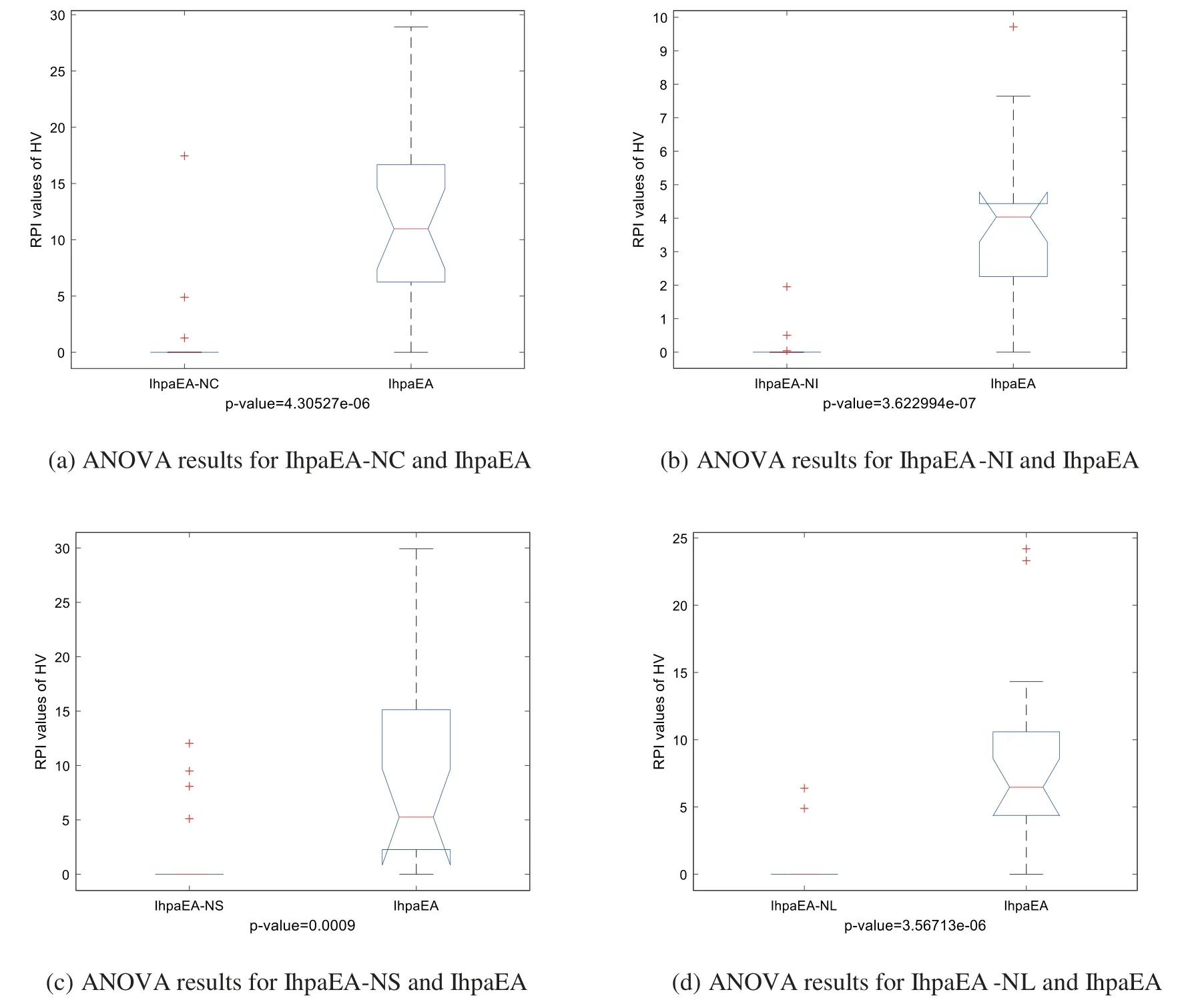
Figure 7:Means and 95%LSD interval for pairs of compared algorithms

From the comparison results given in Table 4, it can be observed that:(1) Compared with the IhpaEA -NC, IhpaEA algorithm obtains 17 better results based on the HV values; (2) the ANOVA results from Fig.7b shows that the IhpaEA obtains significant better results based on the HV results,where thep-value equals to 4.30527e-06(3)for the IGD values,IhpaEA obtains 18 better results;and(4)from the average performance in HV and IGD given in the last line,the efficiency of the proposed crossover heuristic can be verified.

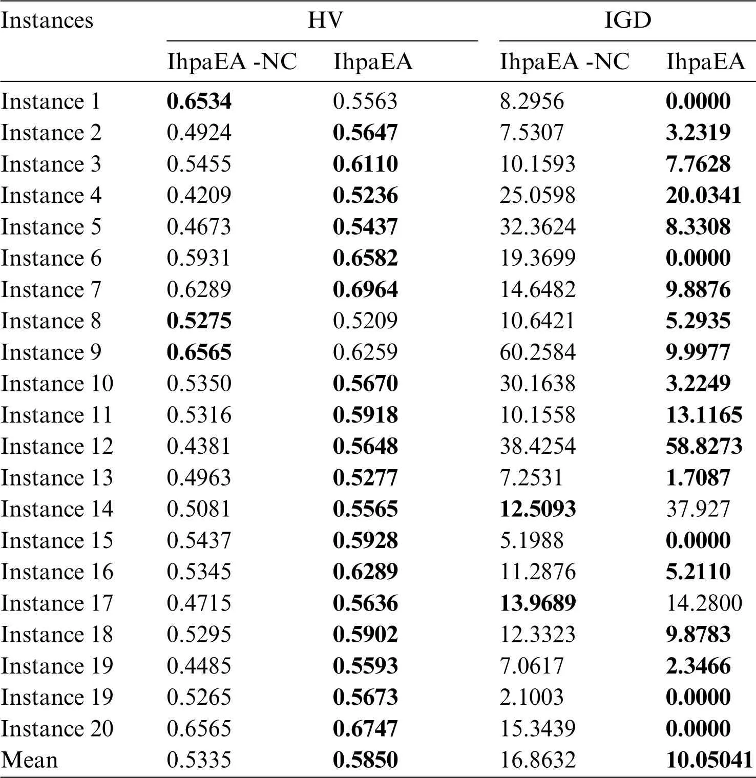
Table 4:Comparisons between IhpaEA-NC and IhpaEA

4.4 Efficiency of the Mutation Operator

Two different types of IhpaEA algorithms are coded to test the performance of the mutation operator discussed in Section 3.6,i.e.,the proposed IhpaEA-NS algorithm without mutation operator,and the IhpaEA algorithm with all the components.

From the comparison results given in Table 5, it can be concluded that:(1) compared with the IhpaEA-NS algorithm, IhpaEA obtains 18 better results, based on the HV values; (2) the ANOVA results from Fig.7c shows that the IhpaEA obtains significant better results based on the HV results,where thep-value equals to 0.0009;(3)for the IGD values,IhpaEA obtains 18 better results;and(4)from the average performance in HV and IGD given in the last line, the efficiency of the proposed mutation operator can be verified.

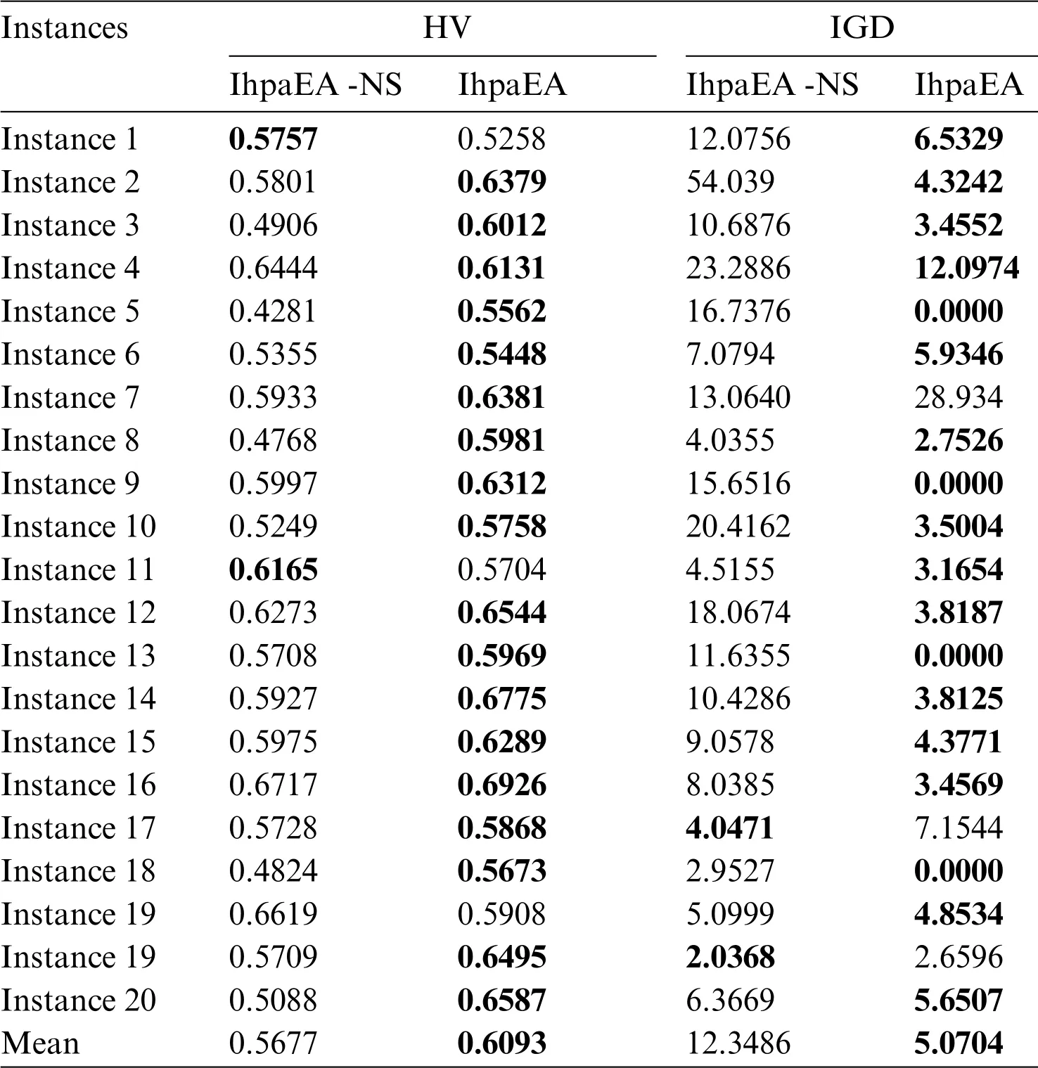
Table 5:Comparisons between IhpaEA-NS and IhpaEA

4.5 Efficiency of the Local Search Operator

To evaluate the performance of the local search heuristic discussed in Section 3.7, two types of IphaEA algorithms are coded:IhpaEA-NL without the local search heuristic and IhpaEA with all components that mentioned in Section 3.7.

From the comparison results given in Table 6, it can be observed that:(1) considering the HV values, compared with the IhpaEA -NL algorithm, IhpaEA obtains 18 better results; (2) the ANOVA results from Fig.7d shows that the IhpaEA obtains significant better results considering the HV results, where thep-value equals to 3.56712e-06 (3) for the IGD values, IhpaEA obtains 20 better results;and(4)from the average performance in HV and IGD given in the last line,the efficiency of the proposed heuristic can be verified.

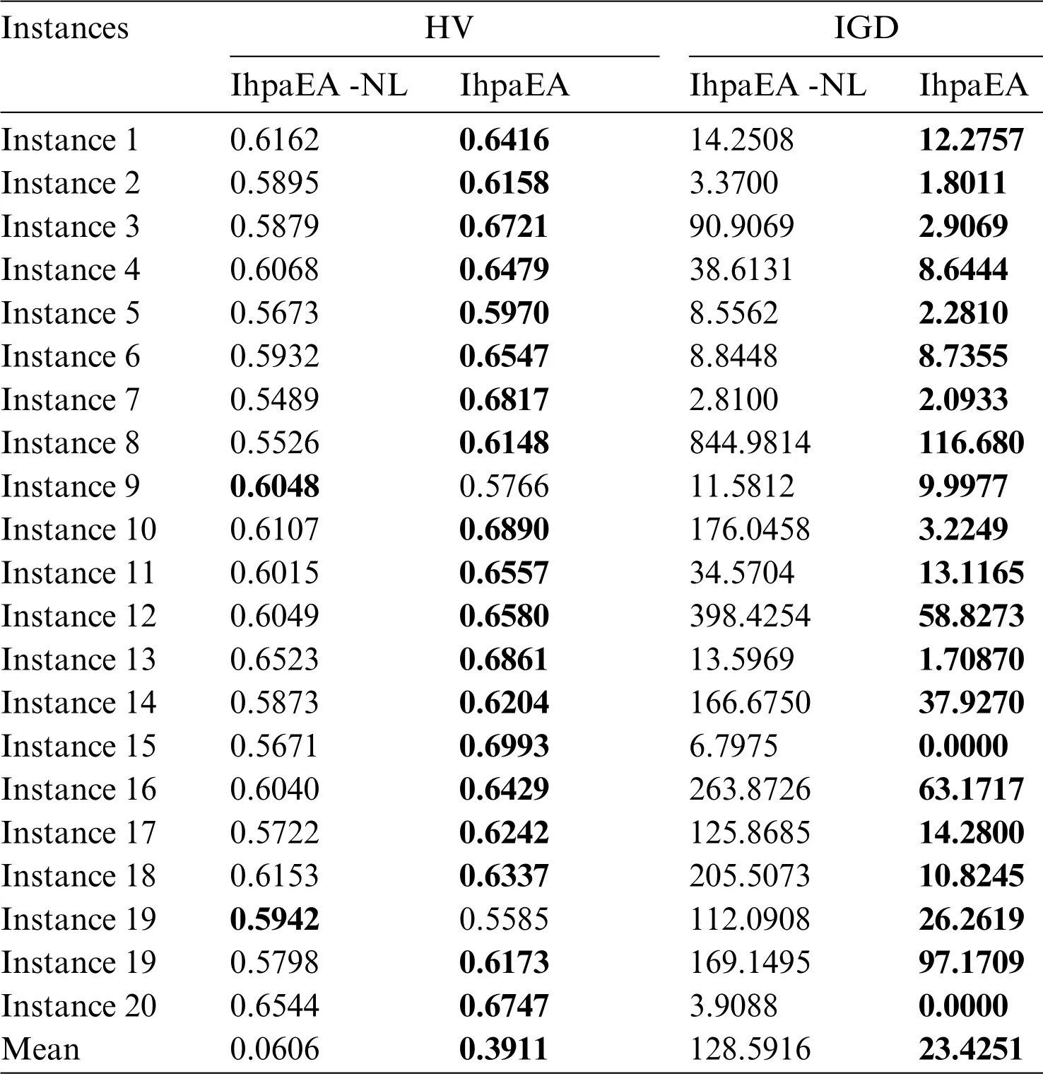
Table 6:Comparisons between IhpaEA-NL and IhpaEA

4.6 Comparisons of the Efficient Algorithms

Three algorithms are selected,namely,NSGAII[37],GFMOEA[38],BiGE[39],to test the effectiveness of the IhpaEA algorithm.Table 7 presents the HV and IGD results after 30 independent runs.

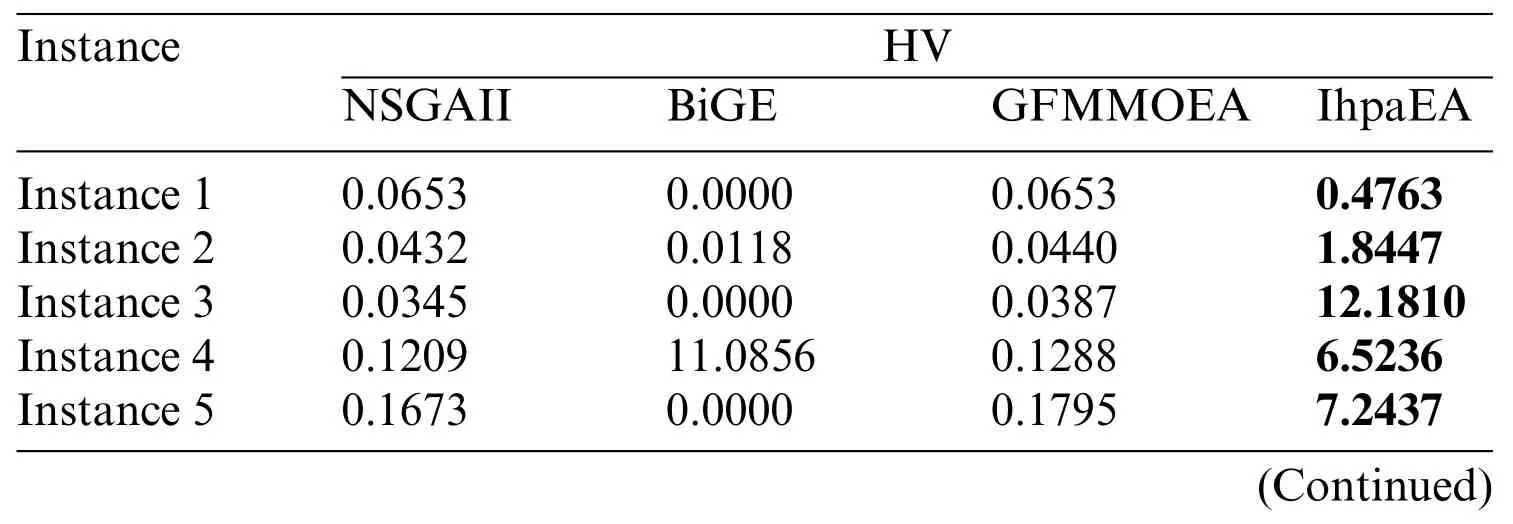
Table 7:Comparisons results of the HV values(NSGAII,BiGE,GFMMOEA,IhpaEA)

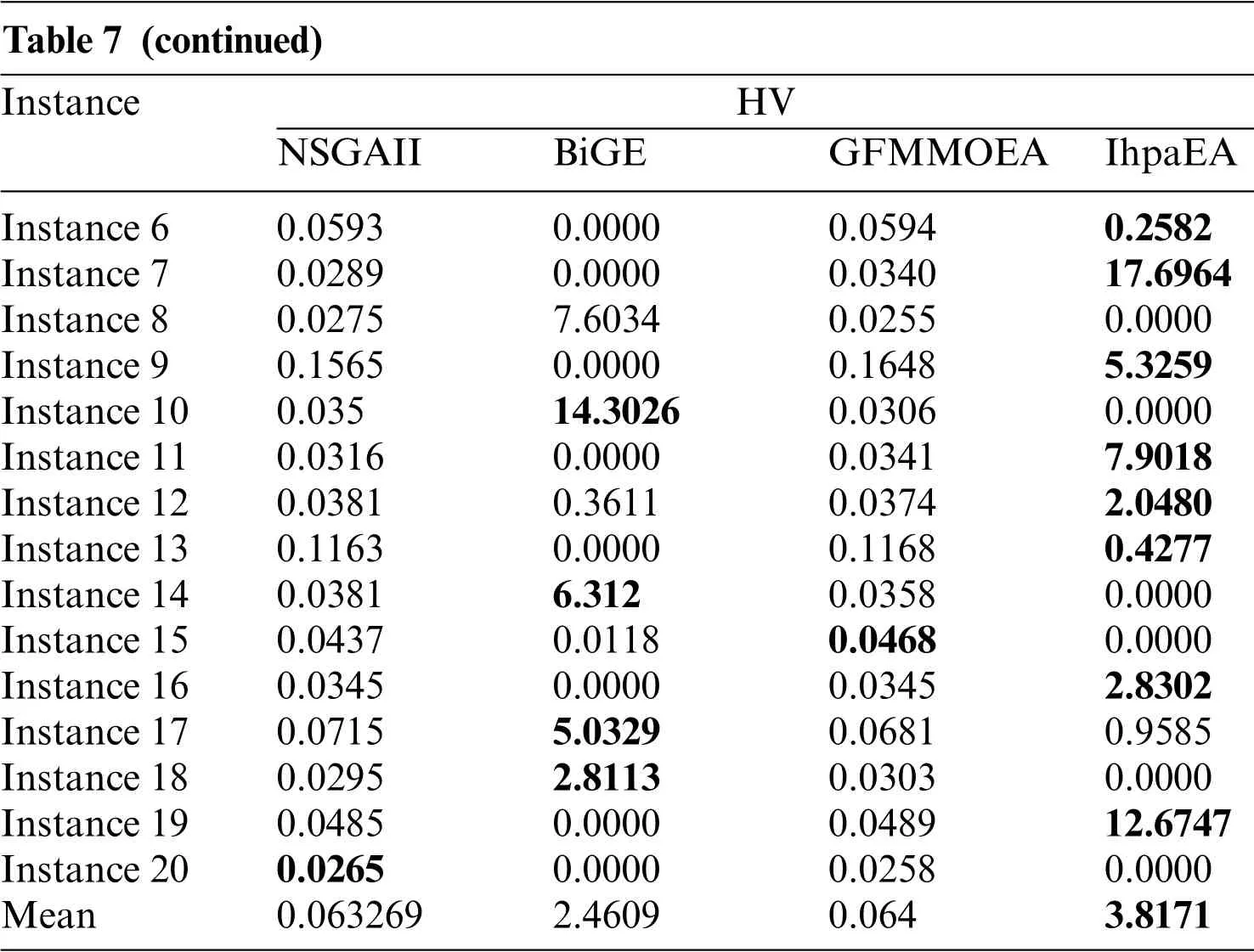
Table 7 (continued)Instance HV NSGAII BiGE GFMMOEA IhpaEA Instance 6 0.0593 0.0000 0.0594 0.2582 Instance 7 0.0289 0.0000 0.0340 17.6964 Instance 8 0.0275 7.6034 0.0255 0.0000 Instance 9 0.1565 0.0000 0.1648 5.3259 Instance 10 0.035 14.3026 0.0306 0.0000 Instance 11 0.0316 0.0000 0.0341 7.9018 Instance 12 0.0381 0.3611 0.0374 2.0480 Instance 13 0.1163 0.0000 0.1168 0.4277 Instance 14 0.0381 6.312 0.0358 0.0000 Instance 15 0.0437 0.0118 0.0468 0.0000 Instance 16 0.0345 0.0000 0.0345 2.8302 Instance 17 0.0715 5.0329 0.0681 0.9585 Instance 18 0.0295 2.8113 0.0303 0.0000 Instance 19 0.0485 0.0000 0.0489 12.6747 Instance 20 0.0265 0.0000 0.0258 0.0000 Mean 0.063269 2.4609 0.064 3.8171

Figs.8a–8c shows the Pareto front charts for solving three different problem scale instances,i.e.,“Instance 1”, “Instance 5”, and “Instance 20”.It can be observed from Fig.8 that, the solutions obtained by the IhpaEA algorithm are close to the Pareto front and well-distributed.

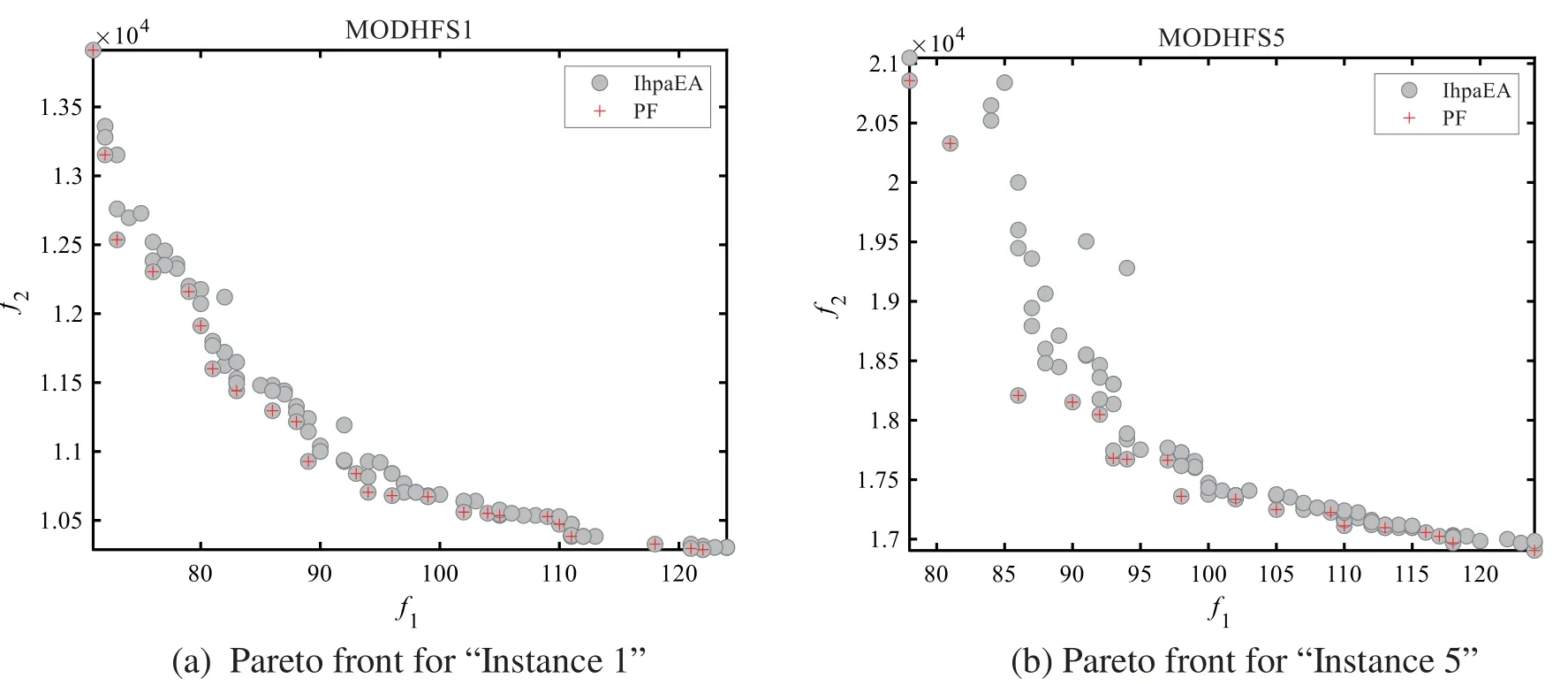
Figure 8:(Continued)

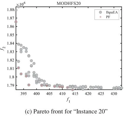
Figure 8:Pareto front results

Table 7 reports the comparison results of the HV values for the given 20 different scale instances.The first column represents the number of the instances.Then, the results collected by NSGAII,GFMMOEA,BiGE,and IhpaEA,are illustrated in the following four columns,respectively.Table 8 reveals that:(1)13 better values obtained by the proposed IhpaEA algorithm for the given 20 instances perform significantly better than other 3 comparison algorithms;and(2)the average values of the last line further evaluate the efficiency of the IhpaEA.In addition,from the compared results of the IGD values reported in Table 8,it can be known that the proposed IhpaEA algorithm gets 19 better values,which further test the superiority of the IhpaEA algorithm.

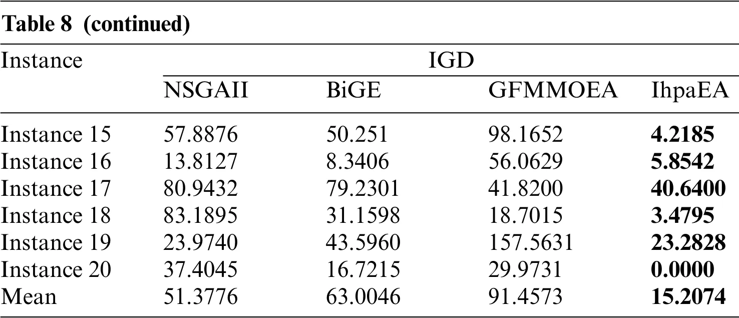
Table 8 (continued)Instance IGD NSGAII BiGE GFMMOEA IhpaEA Instance 15 57.8876 50.251 98.1652 4.2185 Instance 16 13.8127 8.3406 56.0629 5.8542 Instance 17 80.9432 79.2301 41.8200 40.6400 Instance 18 83.1895 31.1598 18.7015 3.4795 Instance 19 23.9740 43.5960 157.5631 23.2828 Instance 20 37.4045 16.7215 29.9731 0.0000 Mean 51.3776 63.0046 91.4573 15.2074

A multifactor analysis of variance(ANOVA)is also performed to verify the difference from the above tables,based on three compared algorithms namely,NSGAII,GFMMOEA and BiGE.Fig.9 reveals the means and the 95%LSD(Fisher’s Least Significant Difference)intervals for the best values of the three compared algorithms.The result of the three comparison algorithms shows statistically significant difference.From Fig.9 we can conclude that the IhpaEA algorithm performs better than other three compared algorithms obviously.

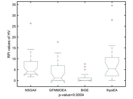
Figure 9:Multi-compare results for NSGAII,GFMMOEA,BiGE,and IhpaEA

Fig.10 shows the Gantt chart for one of the optimal solutions for “Instance 7”.It can be concluded from Fig.10 that the proposed algorithm can obtain some feasible and efficient solutions for the considered problem.

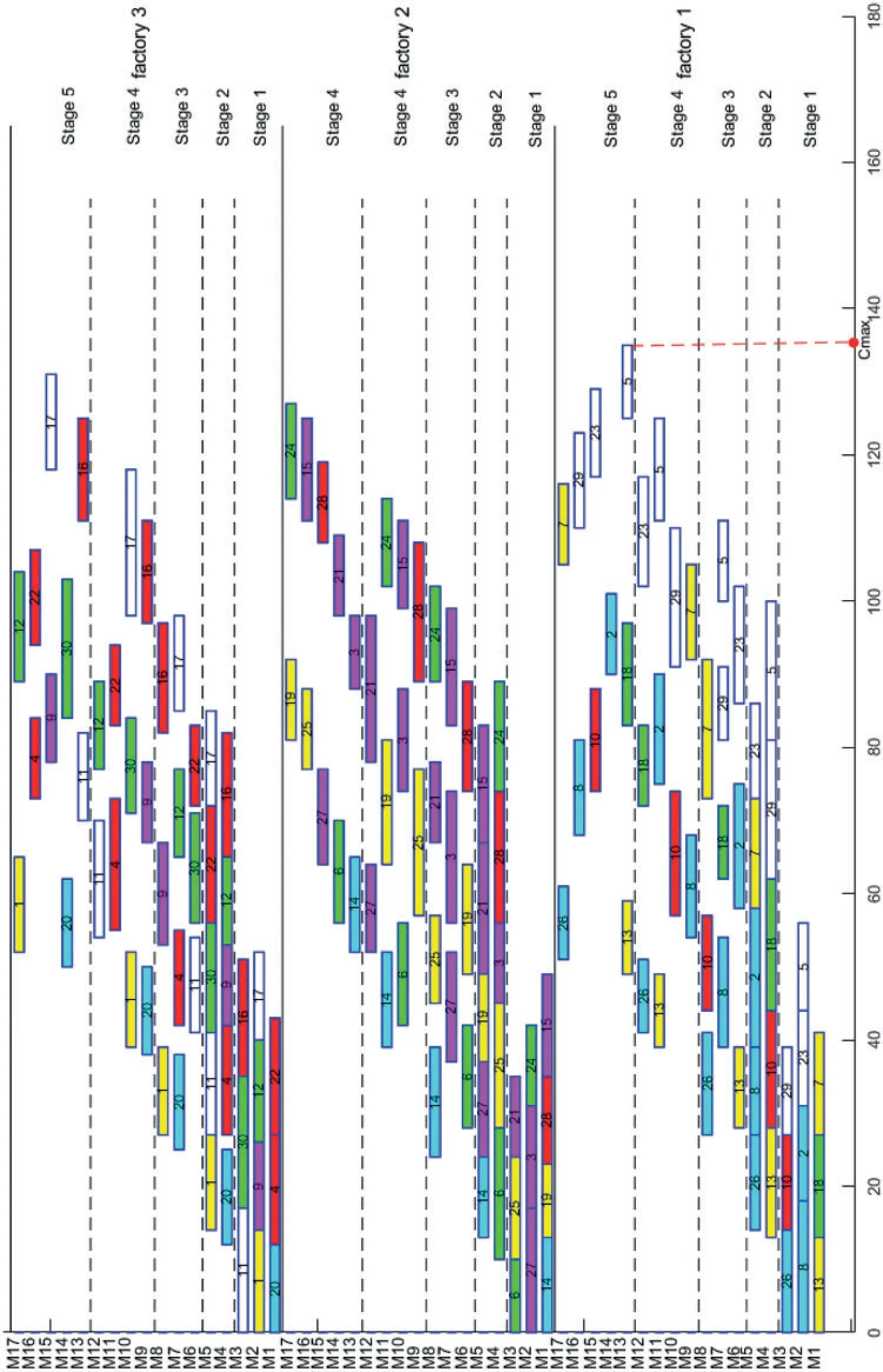
Figure 10:Gantt charts for instance 7

4.7 Experimental Analysis

From the above discussed comparison results,the efficient performance of the proposed IhpaEA algorithm has been tested.The main advantages of IhpaEA are as follows:(1)the proposed initialization heuristic,which can enhance the population diversity and quality;(2)the Pareto-based crossover operator enhance the global search abilities; (3) the mutation operator enhance the convergence of optimization process;and(4)a cooperation of search operators improve the local search abilities.

5 Conclusion

This paper studies a DHFS problem with makespan and total energy consumption.To solving the problem,a multiobjective optimization algorithm is proposed.The contributions are as follows:(1) an efficient encoding and decoding mechanism is embedded; (2) in the initialization phase of the algorithm, considering the constraints in the model, two heuristics are developed; (3) a Paretobased crossover operator is designed;and(4)a cooperation of search operator is developed to further improve the quality of the solution and accelerate the convergence speed of the algorithm.To further illustrate the effectiveness of the proposed algorithm, IhpaEA is compared with three other multiobjective algorithms, including NSGA-II, BiGE, and GFMMOEA, The Pareto frontier is closer to the optimal solution than the other three algorithms.

We test the IhpaEA algorithm with different scales and compare several efficient algorithms with the IhpaEA algorithm.The robustness as well as efficiency is shown by experimental results.There are some works need to be focused as follows:(1) to improve the search capabilities, more local optimization methods or other efficient heuristics need to be introduced; (2) some useful dynamic and rescheduling strategies should be considered in flow shop scheduling problem;(3)more conflict objectives such as maximum workload and parallel batch workload need to be focused on.

Funding Statement:The authors received no specific funding for this study.

Conflicts of Interest:The authors declare that they have no conflicts of interest to report regarding the present study.