Metal Corrosion Rate Prediction of Small Samples Using an Ensemble Technique

Yang Yang,Pengfei Zheng,Fanru Zeng,Peng Xin,Guoxi He and Kexi Liao

1State Key Laboratory of Oil Gas Reservoir Geology and Exploitation,Southwest Petroleum University,Chengdu,610500,China

2School of Earth Sciences and Technology,Southwest Petroleum University,Chengdu,610500,China

3Spatial Information Technology and Big Data Mining Research Center,School of Earth Sciences and Technology,Southwest Petroleum University,Chengdu,610500,China

4Sichuan Xinyang Anchuang Technology Co.,Ltd.,Chengdu,610500,China

5Sichuan Water Conservancy College,Chengdu,610500,China

6CCDC Safety,Environment,Quality Supervision&Testing Research Institute,Guanghan,618300,China

ABSTRACT Accurate prediction of the internal corrosion rates of oil and gas pipelines could be an effective way to prevent pipeline leaks.In this study,a proposed framework for predicting corrosion rates under a small sample of metal corrosion data in the laboratory was developed to provide a new perspective on how to solve the problem of pipeline corrosion under the condition of insufficient real samples.This approach employed the bagging algorithm to construct a strong learner by integrating several KNN learners.A total of 99 data were collected and split into training and test set with a 9:1 ratio.The training set was used to obtain the best hyperparameters by 10-fold cross-validation and grid search,and the test set was used to determine the performance of the model.The results showed that the Mean Absolute Error(MAE)of this framework is 28.06%of the traditional model and outperforms other ensemble methods.Therefore,the proposed framework is suitable for metal corrosion prediction under small sample conditions.

KEYWORDS Oil pipeline;bagging;KNN;ensemble learning;small sample size

1 Introduction

Owing to its economy and safety,pipeline transportation is one of the most important modes of oil and gas transportation[1].However,the longer the pipeline is running,the greater the risk of corrosion[2].Corrosion is the main incentive to increase the risk of oil and gas pipelines [3].Due to the high cost of measuring equipment and the requirements of specific and regular calibration operations,it is not easy to obtain the status of corrosion defect measurement[4].Thus,it is challenging to establish a high-precision corrosion prediction model.Despite this,many scholars have studied this problem and established different corrosion rate prediction models.Traditional(semi-empirical)models include the de Waard[5,6],Cassandra(BP)[7,8],and Norsok[9]models.Of these,the de Waard model has been the most widely used since its establishment, although it rarely considers the influence of protective corrosion, especially at high temperature and pH values.The Cassandra model, on the other hand,takes into account the influence of corrosion inhibitors and can achieve better prediction performance at high temperatures,but it does not consider the influence of medium flow rates and Cl-.The Norsok model is a purely empirical model established using a large amount of data,and takes into account the influence of a greater number of factors compared to the other models;however,as it does not consider the underlying mechanisms,it lacks universality,and it is relatively conservative in its predictions.

With the development of artificial intelligence(AI)technology,the use of deep learning methods to obtain better corrosion predictions for oil and gas pipelines has also become a focus of current research[10–12].For example,Jain et al.[13]proposed a quantitative evaluation model for the external corrosion rate of oil and gas pipelines based on Bayesian networks.Abbas et al.[14] developed a neural network(NN)model to predict CO2corrosion in pipelines at high partial pressures.Ossai[15]developed a feedforward NN based on the particle swarm algorithm(PSO).Chen et al.[16]proposed a fuzzy NN model of Principal Component Analysis Based Dynamic Fuzzy Neural Network(PCAD-FNN).Seghier et al.[4] outlined a new framework of the SVR-FFA model for more accurately predicting the maximum depth of pitting corrosion in oil and gas pipelines.Although these models have achieved high accuracy to a certain extent,such methods are also more demanding with regard to the quality and quantity of pipeline inspection data, which are not always consistent due to the diversity of field conditions and the limitations of inspection technology.As a result,this complicates the process of building models based on deep learning techniques and makes the application and extension of these methods more difficult [17,18].Due to the limitations of data acquisition from real-world pipeline systems,there is a need for high-quality lab-scale experimental data.

Experiments in the dynamic reactor [19] allow corrosion data to be obtained under laboratory conditions; however, such methods tend to be both expensive and time-consuming, and as such can only provide limited data.To overcome the problem of small datasets, some researchers have turned to deep learning methods to obtain reliable prediction models.For example, Zhu et al.and Angshuman Paul et al.[20,21] proposed models applicable to the prediction of image data.Chen et al.[22] proposed the use of an ensemble long short-term memory (EnLSTM) model for timeseries data.Although these models do lead to greater prediction accuracy for small sample sizes,they cannot fully overcome the inherent disadvantages of NN overfitting and weak generalizability [23],which means that such models do not train reliably with small datasets[20].Some studies have found that the use of data mining techniques that build and combine individual learners to form a strong learner capable of better predictions(also known as ensemble learning methods),play an important role in overcoming the overfitting problem[24],and are effectively able to handle data sets with high dimensionality, complex structures, and small sample sizes [25].Such methods are even helpful in solving the problem of unbalanced data distribution[26];as a result,many researchers have directed their efforts toward ensemble learning.For instance, Dvornik et al.[27] demonstrated a significant reduction in the variance by integrating a distance-based classifier in a small-sample setting.Mahdavi-Shahri et al.[24]proposed an ensemble learning method to achieve the best classification results for a multi-label problem with small samples.Guan et al.[28] used ensemble techniques to improve the accuracy of face recognition under small-sample conditions.As the main ensemble learning methods,the bagging(bootstrap aggregation)[29]and boosting[30]algorithms,have been applied in many fields such as predicting cloud meteorological data [31], concrete bearing pressures [32], and the mapping of ecological zones in aerial hyperspectral images[33].Bagging and KNN both perform well in small sample data sets, and scholars [34–36] have also studied the models integrating them.However, it is still worth exploring whether the integrated model can predict small sample data sets of oil industry.Against this backdrop,a proposed framework for predicting corrosion rates under a small sample of metal corrosion data in the laboratory is proposed.The innovations and contributions are as follows:

· Different from other ensemble models, a KNN-based learner’s bagging model is proposed.This model has better performance on the small sample data set of this experiment,obviously outperforming the traditional model.

· The ensemble models of bagging, boosting, and stacking are all used for comparison.In this experiment,bagging is slightly superior to other ensemble models.

· Various factors affecting the experimental results were studied.

Section 2 describes the features of the data involved in the experiment and how to obtain the data.Section 3 introduces the process and method of the experiment.In Section 4,the influencing factors such as data dimension,segmentation rate,and noise reduction processing are discussed,the prediction errors of the integrated model under this data set are compared,and the advantages of the integrated model have been experimented with.Section 5 discusses the experimental results of Section 4.Some primary conclusions are summarized in Section 5.

2 Materials and Experimental Database

For the laboratory experiments in this study,a dynamic reactor apparatus was used(Fig.1),with a solution consisting of 3 L of water obtained from a shale gas gathering pipeline.The operating parameters inside the reactor, including pressure, temperature, and partial pressure of CO2were controlled.In each group of experiments,four samples of the L360 N pipeline(50×10×3 mm3)were used to measure uniform corrosion.The experimental protocol was as follows:firstly, the reactor body and lid were sealed, then the inlet and release valves on the lid were opened and nitrogen gas was passed through for two hours.Next,the release valve was closed and CO2and O2were injected.Finally,once the reactor pressure had increased to 5 MPa through further injecting N2,the inlet valve was also closed.The experimental period was 7 days, and the mass difference of the metal samples before and after the experiment was divided by the reaction time to obtain the average corrosion rate(weight loss tests[37]).Then,the experiments were repeated under different conditions[38,39].Then,the multiphase flow simulation software package OLGA [40] was used to expand the experimental parameters,including liquid flow rate,temperature,inclination angle,CO2partial pressure,and H2S partial pressure,in order to explore the influence of 18 other parameters including flow pattern,flow rate and shear stress on the corrosion rate.The name,abbreviation,unit,minimum/maximum value,average value,and standard derivation(SD)of the experimental data sets obtained by this method are shown in Table 1.

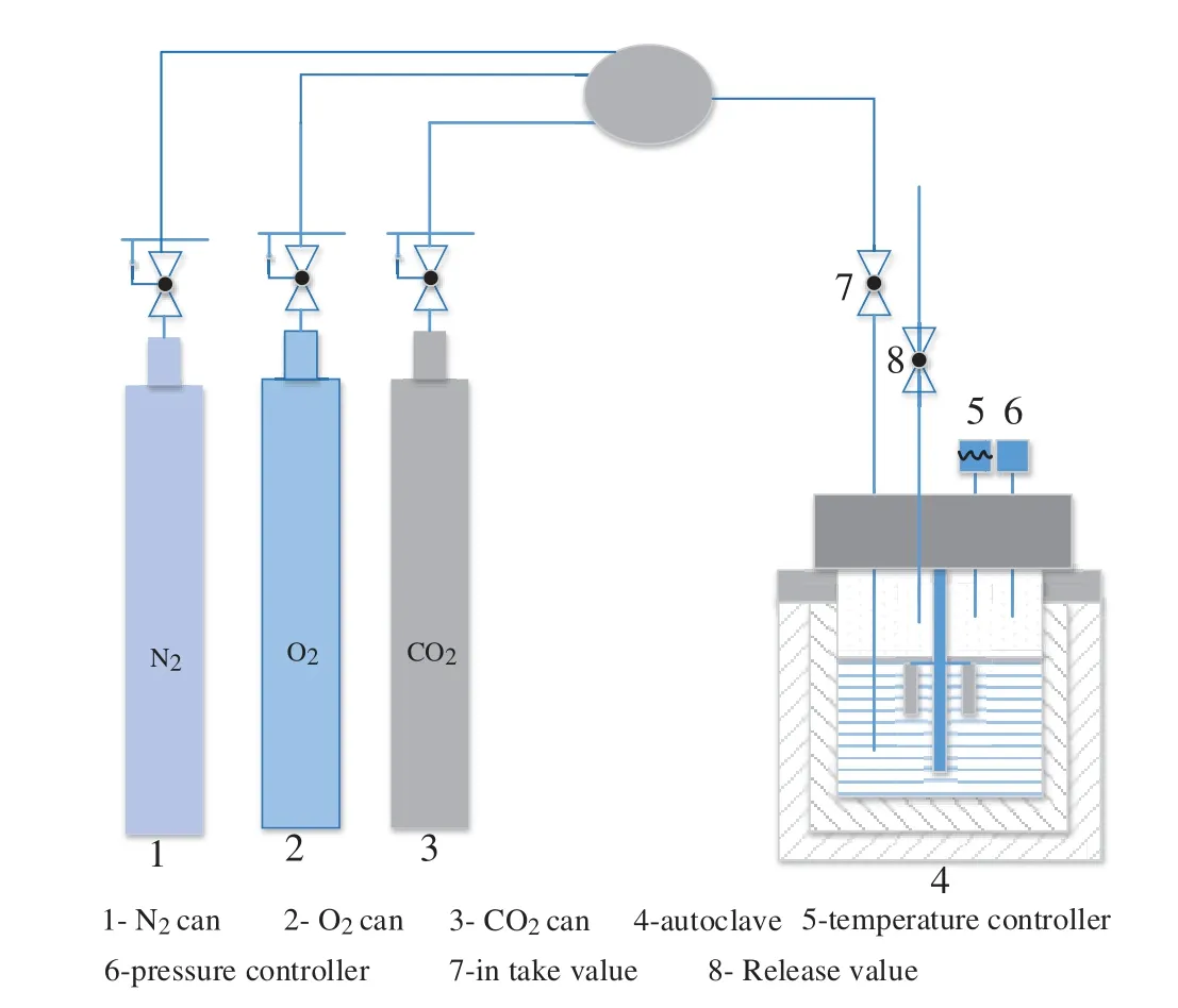
Figure 1:Schematic diagram of the dynamic reactor apparatus[38]

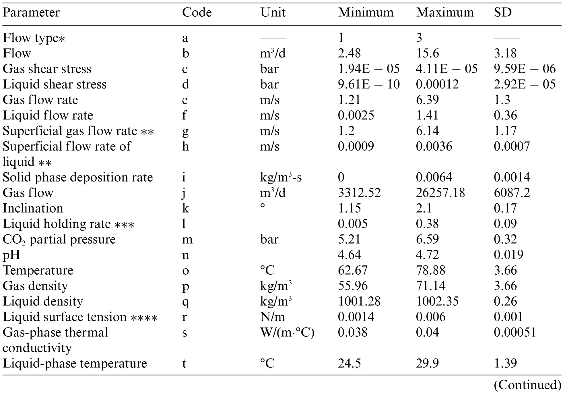
Table 1:Parameters in total in the experimental data sets

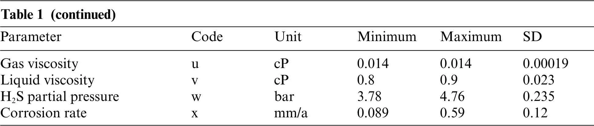
Note:* Flow type:the OLGA classifies flow into four types:stratified flow, annular flow, segmental plug flow, and bubble flow, which were denoted as 1,2,3,and 4,respectively,for this dataset.**Apparent flow rate refers to a virtual(artificial)flow or a single fluid flow velocity(known as the apparent gas or liquid velocity depending on the type of fluid).*** Liquid holding rate is also known as the true liquid content rate or cross-sectional liquid content rate,refers to the proportion of the cross-sectional area of the liquid phase to the total cross-flow area in the process of water and gas flow.****Liquid surface tension:the force that acts on the surface of a liquid to reduce its surface area.

In order to better visualize the correlation between the parameters and the corrosion rate, a Pearson correlation coefficient matrix was drawn (Fig.2).The graph is used to show the linear correlations between parameters, where positive and negative values represent positive and negative correlation,respectively.As shown in the figure,the first five correlations are the solid phase deposition rate and liquid performance flow rate (0.8), the gas flow rate and liquid surface tension (0.78), the liquid density and liquid viscosity(0.77),the partial pressure of carbon dioxide and gas viscosity(0.77),the liquid-phase temperature and liquid viscosity(0.77).

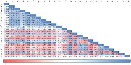
Figure 2:The interaction indices were calculated by interaction detector (big value means strong interaction)

3 Establishment and Methods of the Framework

3.1 Bagging Algorithm

Ensemble learning is a very important area of artificial intelligence and data mining,which aims to build an integrated model by combining individual learners to improve the overall performance[41].In terms of integration approaches bagging and boosting(the adaptive boosting(AdaBoost)algorithm[42] is the most commonly-implemented type of boosting algorithm) are two representative models of ensemble learning.Bagging is one of the first ensemble learning algorithms and uses a parallel integration strategy to randomly select different subsets of the training data.Each subset is then trained based on the same individual learners,and the final prediction results are obtained using a minoritymajority approach for the classification problem and a simple average approach for the regression problem [43,44].The bagging algorithm can improve generalization by reducing the variance error[45].The integration steps are as follows:Suppose we have a training set

The bagging algorithm first resamples the data set,creates a new training subset,and then puts the sampled data into the original data set again.Although this approach may result in some training samples being selected multiple times, while others may not be selected at all, this does not affect the prediction performance of the model.After selecting the individual learning algorithm,put each training subset into the algorithm for calculation.

Combining multiple individual learners to build a learner with stronger predictive ability in the regression problem,the combination strategy is to simply average the prediction results of each weak learner.

In Eqs.(1)–(3),Dis the training dataset,(xi,yi)(i=1,...,m)is the sample in the training dataset,mis the total number of samples,xiis the features of the input data,yiis the label value of the sample,htis an individual learner,Dtis the subset constructed after resampling,tis the number of samples,Lis the individual learning algorithm,H(x)is a learner with stronger predictive ability after integration.

3.2 KNN Algorithm

Individual learners refer to algorithmic models with simple structures.Generally speaking, in the bagging integration strategy,the individual learners are called base learners,and in the boosting integration strategy,they are called component learners[44].For convenience,we collectively call them individual learners.

The main idea behind this algorithm is that the more similar things are,the more likely they are to be adjacent to each other,and it obtains the maximum possibility of the data type of the current point by looking for the data category with the most adjacent data points.This algorithm was chosen because of its simplicity and the ability to distinguish it from other algorithms through the idea of distance sampling[46].The advantage of the algorithm is that it is simple and insensitive to outliers.The disadvantage of this algorithm is that it has high time complexity and spatial complexity,and its interpretation ability is not strong.However,under the condition of small samples,the computational pressure of the algorithm is greatly reduced.Fig.3 shows the forecasting principle of the KNN algorithm.

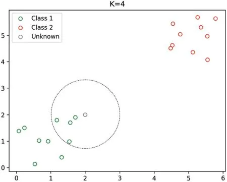
Figure 3:Schematic diagram of KNN(K indicates the number of selected neighbors)[47]

3.3 Framework Building and Experimental Process

Because the model used for comparison has the same construction steps as this framework, we describe its construction process together in this section,and Fig.4 illustrates the overall design flow of this study.

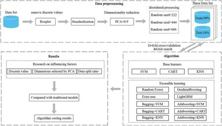
Figure 4:Flow chart of the framework and experimental process

In order to make the model comparison more convincing,we use K-nearest neighbor(KNN)[48],Support vector machine(SVM)[49],and Classification and regression trees(CART)[50]as individual learners for bagging and boosting integration,and in addition,we choose four more mature integrated models of Random forest(RF)[51],Extra tree[52],Gradient boosting[53]and Light gradient boosting machine(LightGBM)[54]for comparison.Based on these four models,our experiments first explored the influence of factors such as eliminating discrete values, reducing dimensions, and changing the proportion of data segmentation on the experiment,which provided the basis for data preprocessing in the framework construction process.

According to the exploration results of the influencing factors,in the aspect of data preprocessing,firstly, according to the corrosion rate, the experimental data set was eliminated by box-plot [55].Considering the different divisions of the training set and the test set under the condition of small samples, the results may be quite different.Before data splitting, three random seeds (222, 444 and 666, respectively) are used for out-of-order processing, to ensure that there are multiple groups of experiments to compare under the same data set.The data was then split into training and test sets at a ratio of 9:1[56],and after the data was uniformly normalized,Principal Component Analysis(PCA)[57]dimensionality reduction was performed to retain more than 90%of the information.

During the process of model building, a combination of 10-fold cross validation [58] and grid search was used to determine the optimal hyperparameter of each model.It was also debugged as a hyperparameter, and the grid search was carried out within a certain range.It was worth noting that we separately search the basic model and the integration method in the grid,and then integrated them according to the selected optimal hyperparameter.Firstly, the training data was divided into 10 subsets on average, of which 9 subsets were used for model training and the rest were used for model verification.This operation was repeated 10 times in a row, the average error was obtained,and then all the parameters in a certain range were traversed by the grid search method.Finally,the parameter combination with the smallest error in 10-fold cross-validation was obtained.The purpose of this process is to achieve the best predictability for each model and to minimize the influence of random seeds on the accuracy of the model.The generalization ability of each model was then tested on the test set and its error was calculated on the test set using mean square error(MSE),mean absolute percentage error(MAPE),and mean absolute error(MAE)metrics,where MSE is the main evaluation index.Finally, the Friedman ranking [59] was used to test the advantages and disadvantages of the model.

To verify the superiority of the model,we also compared the traditional empirical model with the more complex stack integration model and discussed whether the integrated basic learner can improve the performance.

4 Results

This section shows a comparison between the results for the different ensemble learning methods under the conditions of a small sample dataset,followed by the analysis of the effects of discrete values,PCA dimensionality reduction, and data splitting ratio on the prediction.To verify the superiority of the ensemble algorithm approach, the prediction results for the ensemble learning models are compared with those of the weak classifier and traditional models.It is noted that, because of the smaller number of data sets in this experiment, the efficiency of calculation models (e.g., run-time)and not included in the comparison index.

4.1 Ensemble Learning Model Prediction Performance Comparison Results

MSE,MAE,and MAPE were used to determine the error value of the integrated algorithm on the test set.The differences between the predicted and true values of the bagging and boosting algorithms based on MSE are demonstrated in Fig.5.The closer the result is to the diagonal, the smaller the error between the two groups of data.The results show that when the random seeds were 222 and 444,the extra trees,bagging+KNN,and AdaBoosting+SVR models showed the minimum MSE values.However,when the random seed was 666,this changed to bagging+CART,AdaBoosting+CART,and AdaBoosting+SVR.This indicates that the prediction performance of the model changes significantly depending on the training and test sets used.

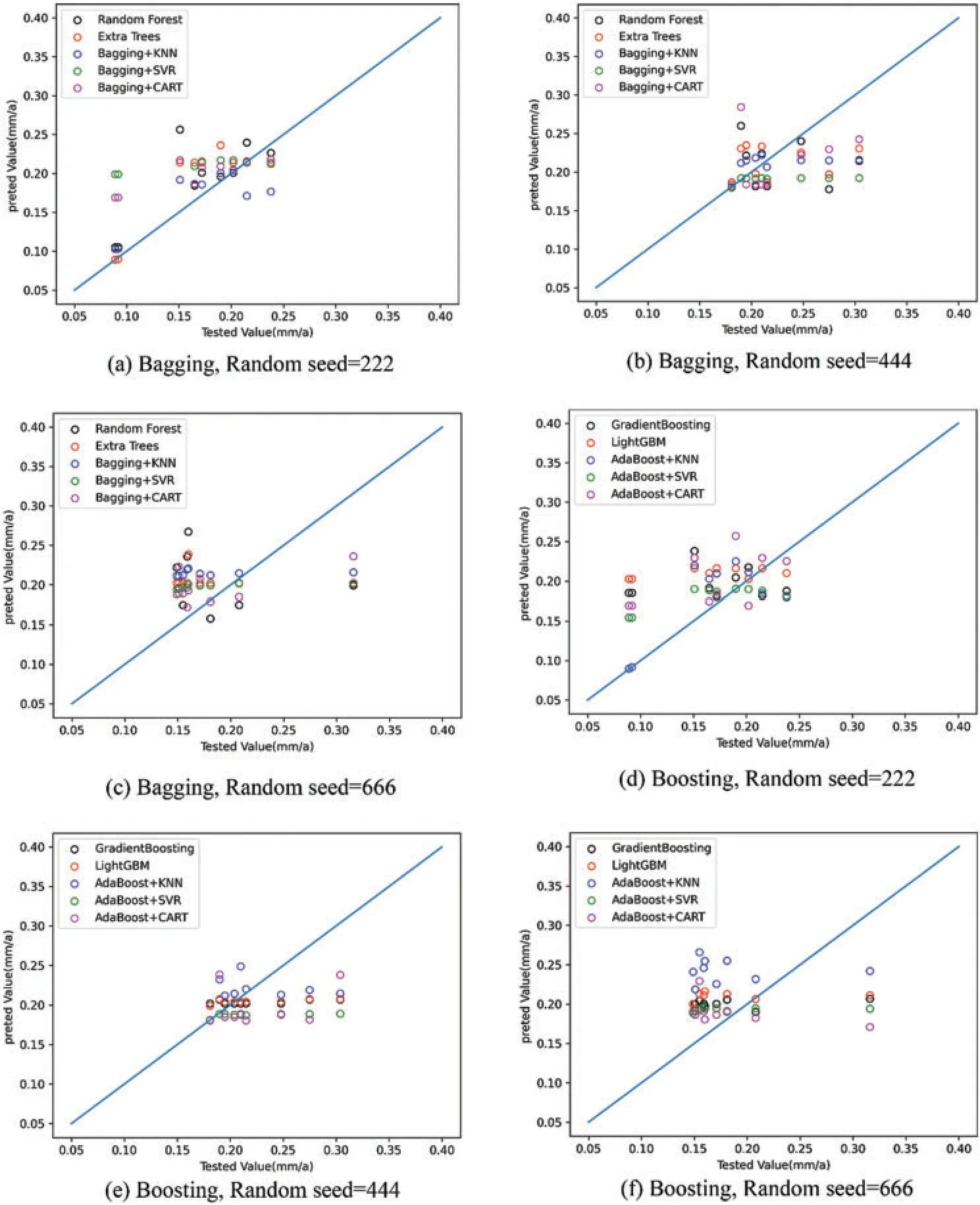
Figure 5:Comparison between model predictions and experimental values

To evaluate the overall performance of each model on multiple datasets,a Friedman ranking plot was drawn(Fig.6).The blue dots in the graph indicate the average ranking of the algorithm,and the farther to the left the numerical value is,the better the model is.The results show that the prediction performance of the bagging + KNN algorithm is the best, followed by extra-trees and bagging +CART,and the prediction performance of random forest was the lowest.The horizontal lines in the figure indicate the allowable fluctuation range of each algorithm ranking.If the horizontal lines of a given pair of algorithms do not overlap each other, it indicates that there are significant differences between these algorithms.However, here, the algorithms in the graph all overlap with each other,indicating that there is no significant difference between them.The order of all algorithms from good to bad is bagging+KNN,extra trees,bagging+CART,adaboosting+KNN,adaboosting+CART,adaboosting+SVR,bagging+SVR,Gradient boosting,LightGBM,Random Forest.

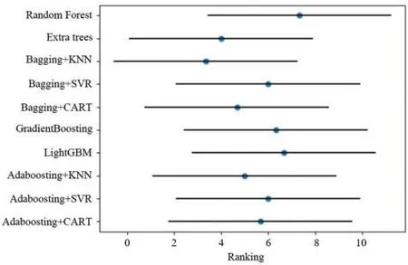
Figure 6:Friedman diagram for the different ensemble learning algorithms

4.2 Experimental Results for Exploring the Influencing Factors

4.2.1 Error Comparison Results after Eliminating Discrete Values

The box-plot uses the quartile as a boundary for analysis of the distribution characteristics of the data,and the data for the corrosion rate term was used as the basis for drawing this plot(Fig.7).The red dashed line in the scatter plot indicates the split line,and the red points represent the discrete points (defined as＞0.42) that need to be eliminated by the box-plot.The total number of discrete points determined using this method is 11.

Among the models used for comparison, we uniformly set their hyperparameters to n_estimators=100 and random_state=222 and set the learning rates of the gradient boosting and LightGBM models to 0.1.Then,the data before and after excluding discrete values were substituted into these models, the results of the 10-fold cross-validation were recorded as shown in Fig.8.The results show that after removing outliers, the average prediction errors of random forest, extra-tree,gradient boosting,and LightGBM algorithms are reduced by 64.16%,68.50%,62.88%,and 63.81%,respectively.This shows that the use of box-plot to eliminate discrete values can help improve the prediction performance of the model.

Figure 7:Scatter plot and edge box-plot of the corrosion rate

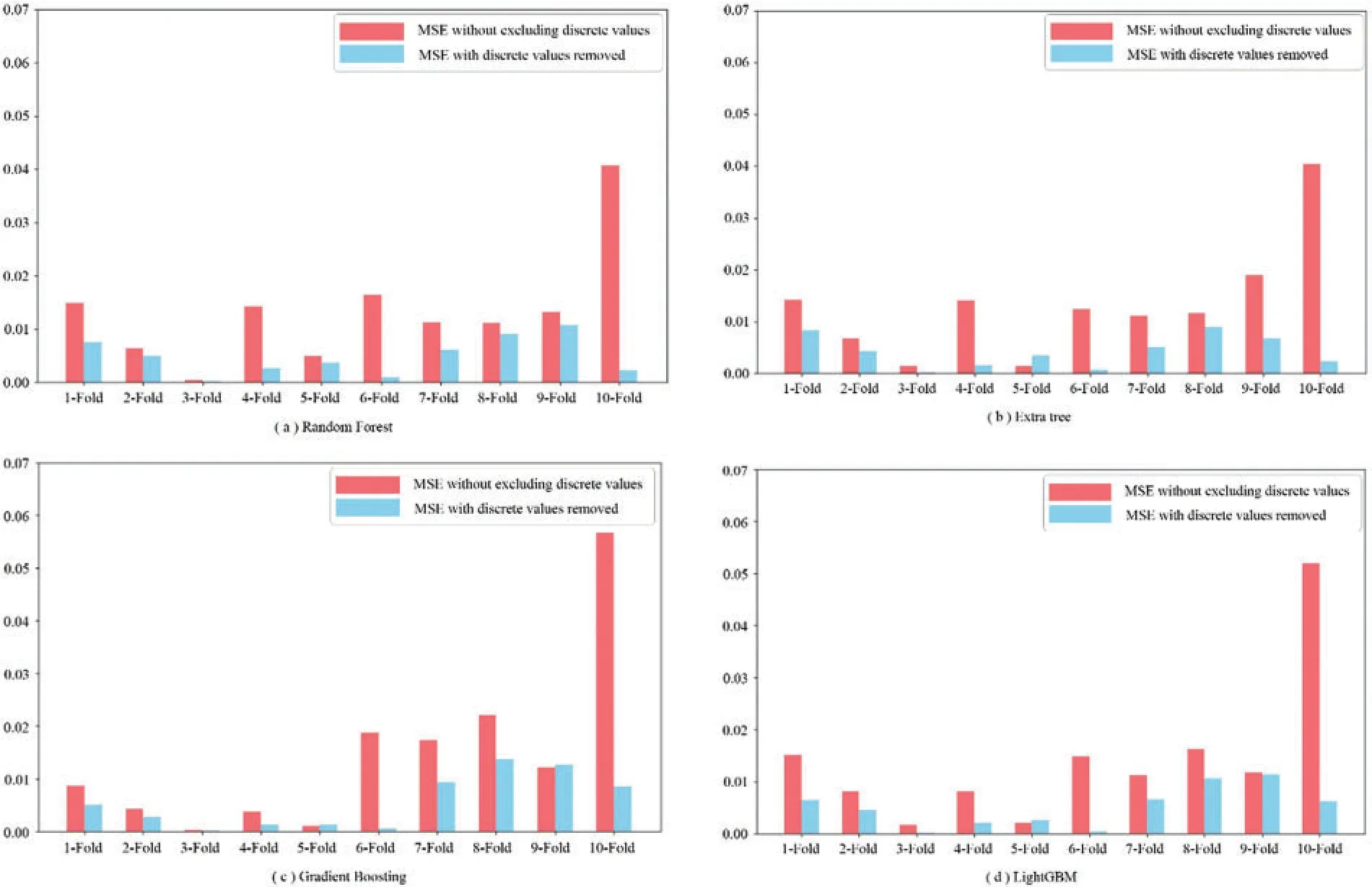
Figure 8:10-fold cross-validation histograms before and after removing the discrete values

4.2.2 Error Comparison Results after Using PCA to Reduce the Dimensionality

In general, although the dataset needs multiple dimensions of features to be characterized as exhaustively as possible,it is not always advantageous to have more features,as the presence of some features may cause the prediction result to drop.In other words,some poorly correlated parameters can be removed[60].In this data set,the percentage of each principal component,wherein the information interpretation rate of the first principal component is 55.68%,and the corresponding cumulative sums of principal components are the sums of the first 14,11,and 8 principal components when 95%,90%,and 85%of the information is retained,respectively.

In this part, only the dataset with an out-of-order seed of 222 was selected when the data was split, and PCA was used to divide this dataset into three-dimension data with dimensions retaining 95%, 90%, and 85% of the information.The hyperparameter involved in the model was set to random_state=222, and the learning rate of the gradient boosting and LightGBM was 0.1.19 numbers from 10 to 200 were moderately spaced, and these numbers were set to n_estimator.Finally,the evaluation value of the predicted results of these models was used as the basis for model comparison.Fig.9 shows the results of the calculations when no principal component scaling is used.Table 2 shows more details.This shows that the error value is significantly higher when the proportion of principal components was selected as 95%as opposed to 90%and 85%;further,the error values for the latter two cases are similar,except that the MSE value of the extra tree model with 90%principal components(0.001545)was smaller than that with 85%principal components(0.002592).Therefore,although PCA is a commonly-used method for achieving data dimensionality reduction under small sample conditions, there is no uniform standard for how much information should be retained in different scenarios,and 90%was found to be the optimum value in this study.

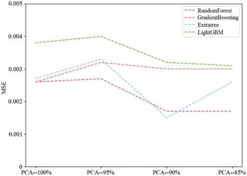
Figure 9:Prediction error of each model after PCA dimensionality reduction

4.2.3 Error Comparison Results for Different Data Segmentation Ratios

Different models were used to compare the results of the prediction errors for different split ratios.As shown in Fig.10 and Table 3,the results show that when the split ratio is 9:1,these models predict the minimum average error, where the MSE average of RF is 0.0017, Gradient Boosting is 0.0026,Extra tree is 0.0024,and LightGBM is 0.0025.When the split ratio is 8:2 and 7:3,the performance on different models is also different.

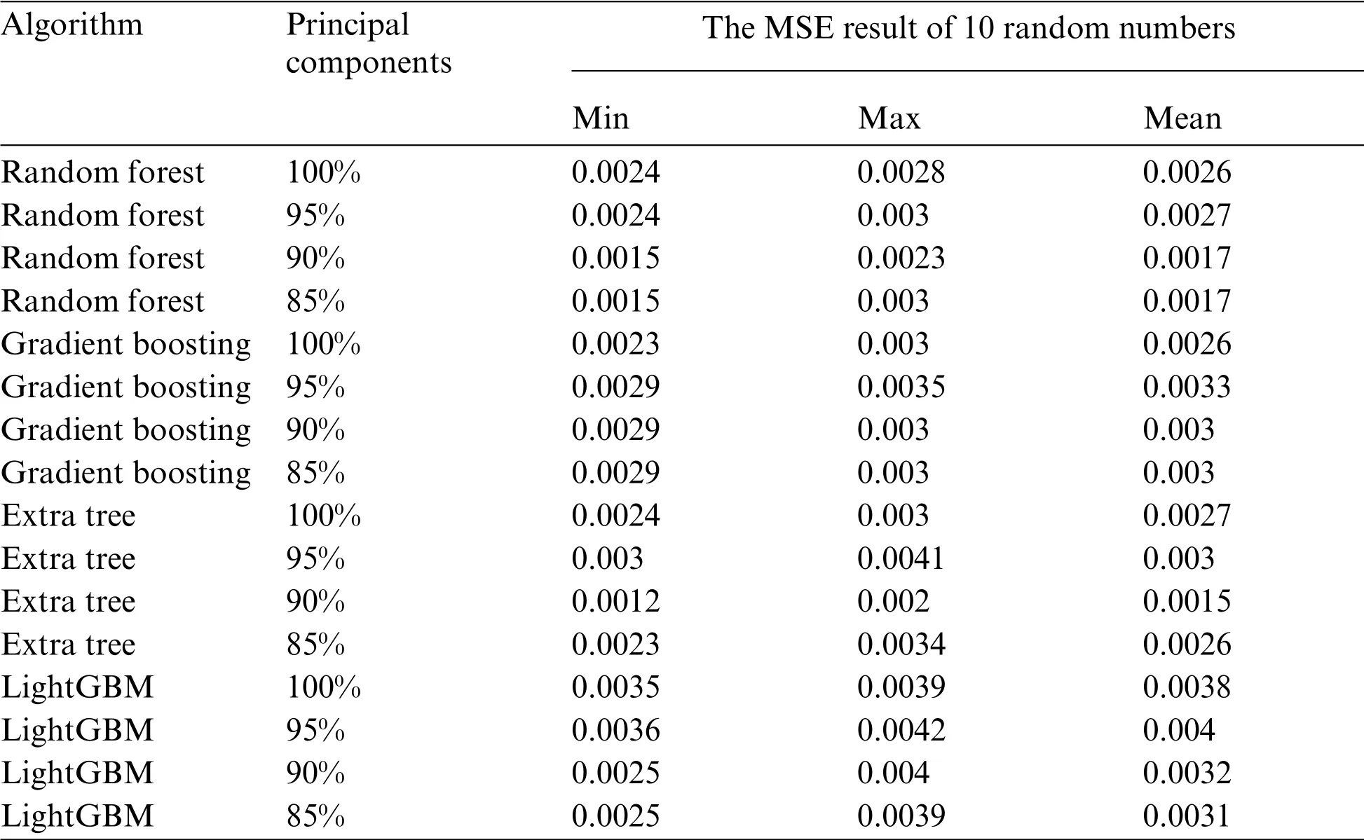
Table 2:MSE results for the different principal components

Figure 10:Prediction error of each model under different split ratios

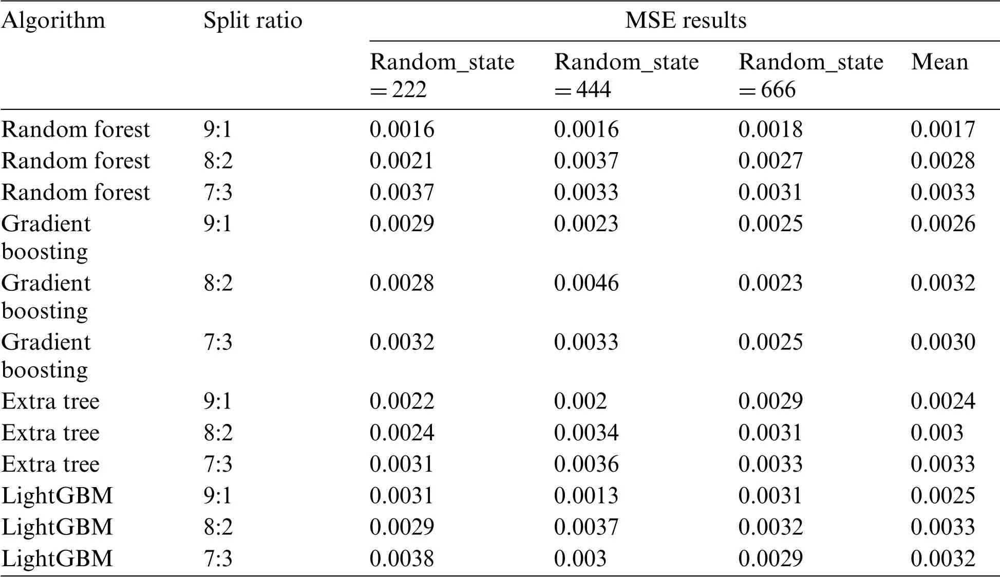
Table 3:Detailed parameter values of MSE results for different split ratios

4.3 Comparison Results of Prediction Errors between Individual Learners and Ensemble Models

To investigate whether the ensemble learning models performed better than the individual learners, the results of integrating the individual learners KNN, SVR, and CART with the bagging and AdaBoosting algorithms were compared in three randomized segmentation experiments(Fig.11).These results show that the bagging algorithm reduces the MSE error values when the individual learners are KNN and the random seed is 222 or 444, while AdaBoosting increases the error value under all three random seeds;further,when the individual learners are SVR,except for the case with a random seed of 666,AdaBoosting significantly reduced the error,and in other cases,bagging and AdaBoosting had similar error values as the individual learners.However,when the individual learners are CART and the random seed is 444 or 666,both bagging and AdaBoosting reduce the prediction error values,while the opposite is observed for a random seed of 222.

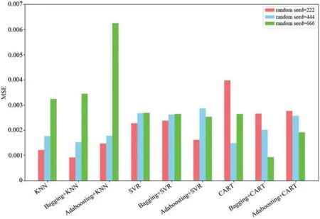
Figure 11:Comparison of the MSE values of different algorithms

4.4 Comparison Results of Prediction Errors between Ensemble Methods and Traditional Models

A traditional model for oil and gas pipeline corrosion rate prediction,the de Waard model[5,6],is given by the following equations:

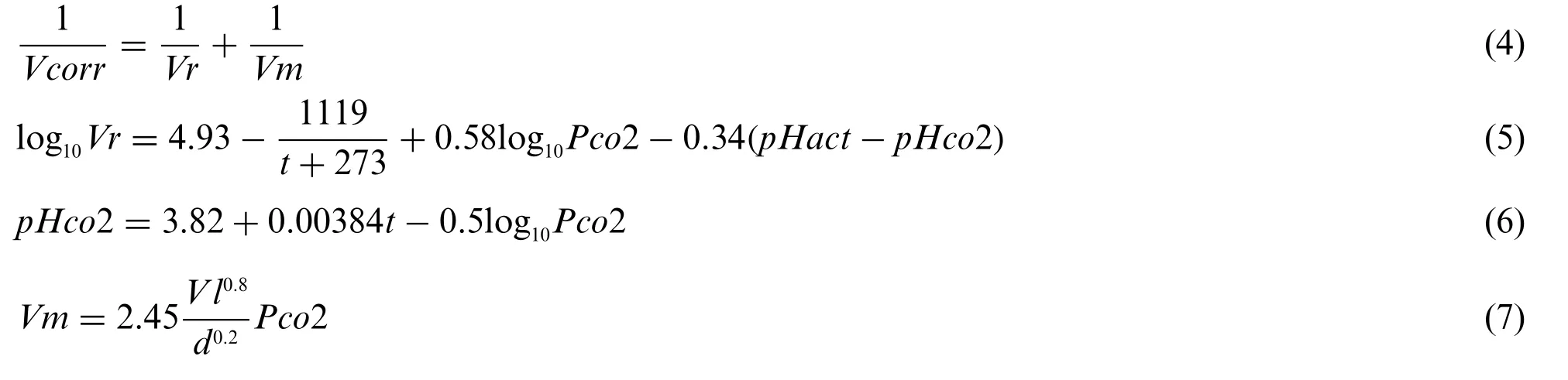
In contrast to the de Waard model, the Norsok M506 model [9] uses different equations over different temperature intervals.In the temperature range from 20°C–150°C,the model is given by:

Between 15°C–20°C,the model is given by:

Between 5°C–15°C,the model is given by:

In Eqs.(4)–(10),Vcorris the corrosion rate in mm/a,Vris the reaction rate in mm/a,Vmis the mass transfer rate in mm/a,tis the media temperature in°C,Pco2 is the CO2partial pressure in MPa,pHactis the actual pH,pHco2 is the pH of CO2-saturated solvent,Vlis the liquid phase flow rate of the medium in m/s,dis the pipe diameter in m,fco2 is the fugacity of CO2,Ktare temperature-dependent constants,τwis the wall shear force in Pa,andf(pH)tis the pH-dependence term.

As the parameters of the de Waard model include the pipe diameter,the effect of which cannot be measured under laboratory conditions,the Norsok M506 model was selected as the control model for this study, as it is a purely empirical model based on a large amount of experimental data.The remaining data after the exclusion of the discrete values were selected for the comparison of prediction results,and the MAE value was used as the performance metric.For the ensemble learning algorithms,the average values of MAE for each model under three random seeds were compared.Fig.12 shows that the MSE error value of the bagging+KNN framework recommended in this study is only 0.0346,while the error value of the traditional Norsork M506 model is 0.1322.This framework is also slightly better than other ensemble models.

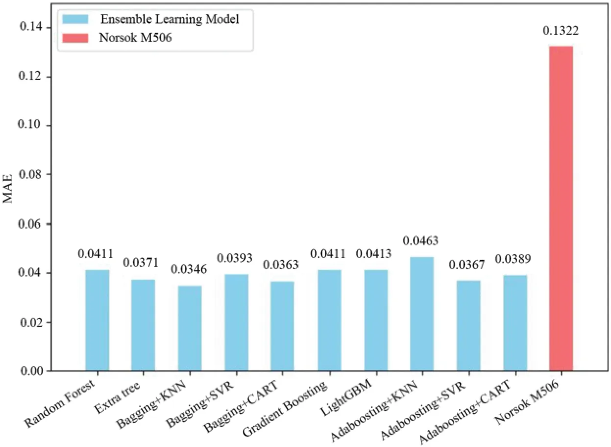
Figure 12:Error comparison results between the traditional and ensemble models

4.5 Comparison Results of Prediction Errors between Ensemble Methods and Stacking Models

The Stacking [61] model allows any combination of different types of models.The integration strategy is to first use the K-fold cross-validation method on the original data to predict the model that needs to be integrated.After obtaining the predicted value of each integrated unit, the average value of the predicted results is used as input into a simpler prediction model(the purpose of this is to prevent overfitting),and the predicted value is the final result.The ensemble units of this ensemble model are usually selected as bagging model and boosting model.In this section,a total of 11 ensemble models(with the addition of the XGBoost[62]model)were used as base models to be integrated into the Stacking mode,in this experiment,to control the number of combinations,each model was only used once.Fig.13 shows the prediction errors under different combinations.From this figure,it can be seen that with the increase of the number of combinations,the prediction error values become more concentrated,and almost every segment has similar error variation rules.Table 4 shows the minimum values of MSE for different combinations and the percentage of their predictions that are improved(relative to the models involved in the combination).When the random splitting seed is 666, under the premise that the prediction error of the basic model is larger, the integrated prediction error is further enlarged,which leads to the fact that the prediction performance of almost all models hardly improves under this data set partition condition.If only the random splitting seeds 222 and 444 are analyzed,as the increase of integration times,the probability that the prediction effect after integration is better than that of a single sub-model will gradually decrease.These results show that even if there is a combination of better prediction effects in stacking,regardless of the prediction performance of the model or the proportion of prediction performance improvement,the stacking integration mode is not very suitable for small sample prediction under this data.

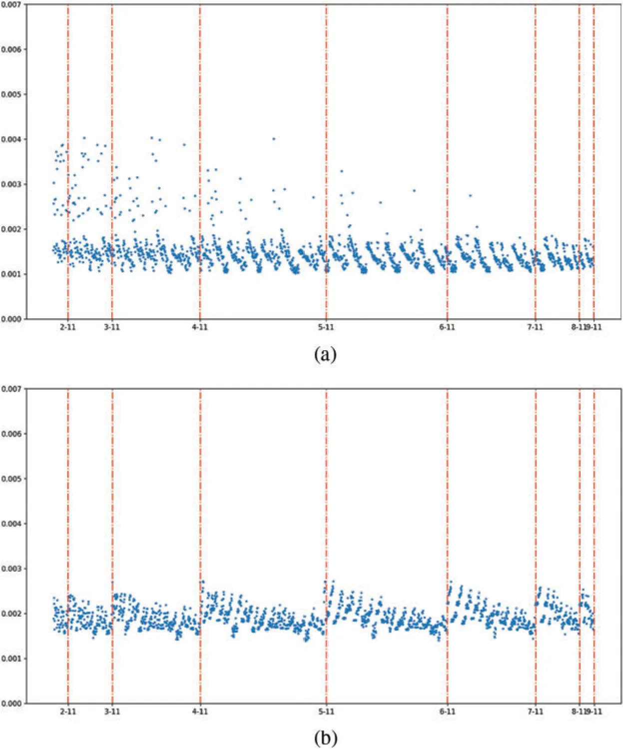
Figure 13:(Continued)

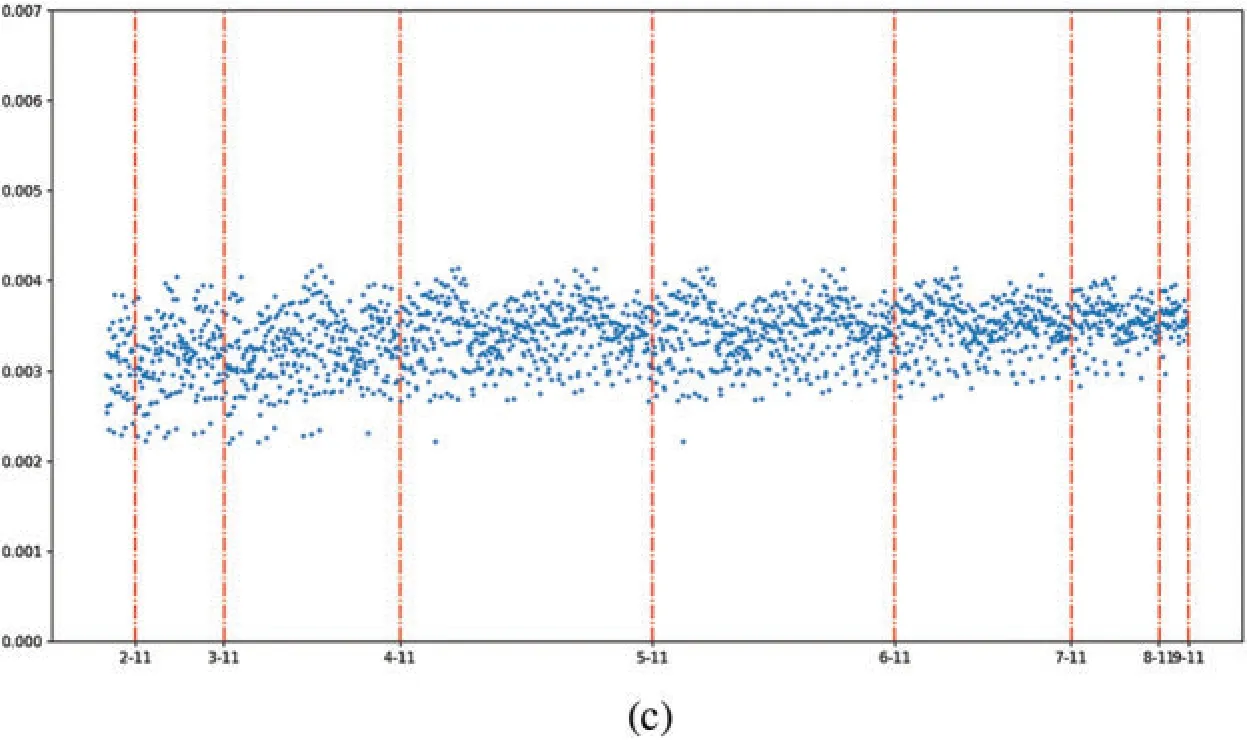
Figure 13:Combined prediction error plot in stacking model.a, b, c indicate the prediction results when the random splitting seed is 222,444,666,respectively;the horizontal coordinates of the graph indicate the number of models involved in the combination

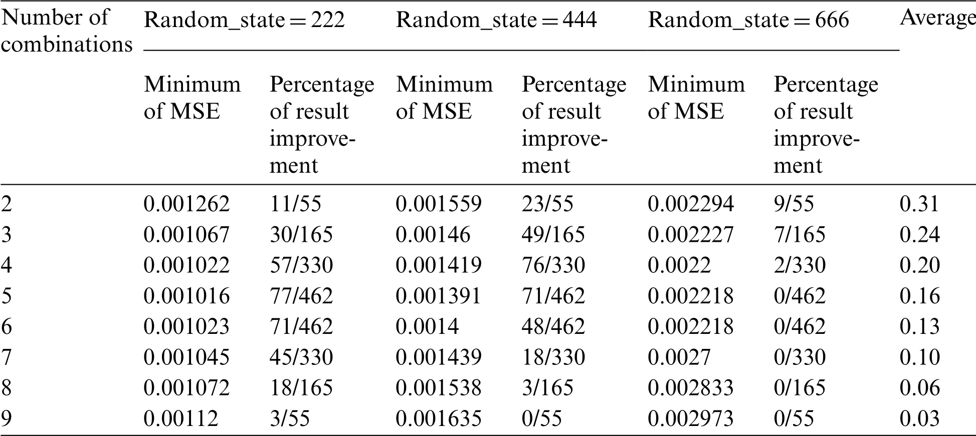
Table 4:Comparison table of prediction performance of each combination in Stacking model

5 Discussion

5.1 Predictive Performance of the Framework

In this study, the ensemble learning algorithms with the smallest MSE were found to be bagging + KNN,extra trees,and bagging+CART,which were all based on the bagging framework.This shows that the bagging algorithm is superior to boosting algorithm in small data set prediction.The results obtained here are consistent with Wang et al.[44], those who found that the bagging method was superior to boosting method in classification,and the former performed relatively better in the presence of noise.However, when using ensemble learning to analyze remote sensing images,Both Chan et al.and DeFries et al.[63,64]found that the AdaBoost algorithm had higher accuracy and that the bagging algorithm is more stable.The reason for the differences between the aforementioned studies and the present study is that in the latter, there are some instances where the discrete values(i.e., noise) are not completely removed, which is more detrimental to boosting methods [65].The differences between the optimization strategies of the two algorithms also contributed to their different prediction performance.The bagging algorithm uses a parallel strategy to average the errors of some discrete values while boosting uses a serial strategy to increase the weight of the discrete value errors present in the training set during the optimization process.It is worth noting that among different models, the random forest algorithm has the lowest prediction rank, which is mainly due to the large prediction error of the last random seed.Bagging + KNN framework has achieved the best prediction results, but under the condition of small samples, data plays a vital role in the results, so the performance of other data sets is still worth exploring.

5.2 Exploratory Analysis of Influencing Factors

In this experiment, the prediction error of each model is reduced after the discrete values are eliminated, because when the amount of data with some special features is small, the distribution of these data relative to other data forms a small disjunctive area which may not be visible [66,67];Therefore,it is not easy to determine whether the values in these areas are true values or noise[68],and the existence of such values leads to insufficient support of the prediction bounds, making it more difficult for the learning algorithm to achieve good generalization [26].Therefore, excluding these values not only reduces the number of small intermittent areas but also has a positive impact on the model’s generalization (the model’s generalization is inherently weak under the condition of small samples).Admittedly, the model fitting in this study has some defects in the elimination of discrete value.Discrete rejection based on corrosion rate alone would have resulted in the incomplete rejection of discrete values as well as possible rejection of non-discrete values.The reason why this culling is not based on the feature values is that the data set has multiple dimensions, and discrete culling of each feature may lead to a small sample size,thus leading to a larger prediction errors.In the model applicability evaluation,when the random seed of the control partition is 666,the prediction error increases significantly,which is likely due to the discrete values in the test set being mixed with those that have not been removed.Therefore,when the study sample is small,more rigorous rules for determining the discrete values should be established.In addition,when building a prediction model based on small data set,when summarizing the model,the verification data should be kept as small as possible with respect to the training set.

The research shows that dimension reduction is helpful to improve the prediction accuracy of the model.In our experiment,when 90%of the information dimension are retained,the prediction effect is the best,while when other information dimensions are retained,the result fluctuates greatly.This shows that although PCA is a common method for dimensionality reduction of small sample data[69],there is no uniform standard for how much information should be retained in different scenarios,which should be selected according to the actual situation.

In the experiment of the influence of segmentation ratio on the prediction error, we found that with the decrease of the training set ratio,the prediction error becomes larger.This is because when the number of training sets decreases, over-fitting is more likely to occur, which will lead to poor generalization ability of the model.This is consistent with the current mainstream research [67], so whether it is a small sample condition or not,increasing the amount of training data will always help to predict the results.

5.3 Comparison with Other Models

Although many researchers believe that ensemble learning is superior to individual learners and helps solve small-sample problems[27],the results from Fig.11 shows this is not necessarily the case.Windeatt[70]put forward that,to obtain a good integration,the conditions of accuracy and diversity must necessarily be satisfied.Therefore,when the dataset is small and contains some discrete values,ensemble learning methods should not be used blindly.In such cases,if the bagging algorithm is not able to achieve good prediction results,it is worth trying individual learners.

Fig.12 shows that the predicted MAE value of the Norsok M506 model was 0.1322, which is significantly larger than that of the ensemble learning algorithm.This indicates that ensemble learning still performs better than traditional empirical models even under small sample conditions.In this case,the results from the Norsok M506 model are relatively conservative compared to other traditional models,which results in larger predicted corrosion rates and thus higher prediction errors[9].

The results of Fig.13 show that the floating range of the prediction error becomes smaller as the number of combinations increases in the Stacking combination model.This means that if one wants to integrate with the Stacking model,it is not better to have more model combinations,rather a smaller number of combinations is more likely to make the combined prediction error decrease.In most cases of this part of the experiment, the prediction performance after using the stacking combination did not outperform the prediction performance of the underlying ensemble model,indicating that using the Stacking algorithm does not further improve the predictive power of the model.As stated by other researchers [71], improving prediction performance using Stacking models requires that the models involved in the integration are differentiated and have good performance,and these conditions cannot be met in the small sample condition.The results in this section show that although the prediction error values of the bagging + KNN framework are still largely under small sample conditions, it is more suitable for prediction under small sample conditions than the traditional model and the more complex Stacking model.

6 Conclusions

In this paper,a bagging ensemble framework based on knn-based learners is proposed to predict metal corrosion rates under small laboratory sample conditions in the absence of real oil and gas pipeline data.The two most important steps in the experimental preprocessing step are PCA dimensionality reduction and boxplot-based removal of discrete values.These two steps are aimed at optimizing the data set and reducing the influence of extraneous factors and noise on the experiment.

99 data sets are used for training and testing at the ratio of 9:1.Based on this data set, other models are compared and analyzed.The results show that when the MAE value of the Norsok model is 0.1322, the error of the bagging + KNN framework is only 0.0346, and the error value of this framework is slightly smaller than that of other integrated models,indicating that this framework has certain advantages in the scene.The stacking mode is more complicated but the prediction effect is not ideal,so it is not recommended to use stacking under the condition of small samples.In addition,the effect of only using the individual learner as the prediction model in this experiment is not as bad as imagined,so when the performance of the computing equipment is poor,and the prediction results of the integrated model are not ideal,you may try the individual learner.

The effects of various factors on the experimental results are discussed.The results show that using box-plot to remove discrete values and reduce the dimension moderately (the best result in this experiment is to keep the dimension of 90%information),and increasing the number of training samples can improve prediction performance to some extent.In addition,our research found that the error value of bagging mode is often smaller than that of Boosting mode in the small sample scenario of this experiment,which indicates that bagging has greater advantages in this scenario.

Although the performance of the proposed framework on this data set is better than that of other models, there is still a large error value on the test set, so the generalization ability of this model is still worth discussing.Under the condition of small samples,slight changes of data may cause a great interference to the results,so this framework only provides an idea to study the corrosion of oil and gas pipelines under the condition of small samples.It is worth noting that the framework removes discrete values and reduces the fluctuation range of the data set, so its generalization ability will be limited when it is used to verify new data sets.Therefore,for future researchers,it is very important to explore the effect of removing outliers in small samples in more detail and how to improve the generalization ability of the model.

Availability of Data and Materials:The data that support the findings of this study are available on request from the corresponding author.The data are not publicly available due to privacy or ethical restrictions.

Funding Statement:This work was supported by the National Natural Science Foundation of China(Grant No.52174062).

Conflicts of Interest:It should be understood that none of the authors have any financial or scientific conflicts of interest concerning the research described in this manuscript.