Stability Analysis of Landfills Contained by Retaining Walls Using Continuous Stress Method

Yufang Zhang,Yingfa Lu,Yao Zhong,Jian Li and Dongze Liu

1China Academy of Railway Sciences Corporation Limited,Beijing,100081,China

2School of Civil,Architecture and Environment,Hubei University of Technology,Wuhan,430068,China

ABSTRACT An analytical method for determining the stresses and deformations of landfills contained by retaining walls is proposed in this paper.In the proposed method,the sliding resisting normal and tangential stresses of the retaining wall and the stress field of the sliding body are obtained considering the differential stress equilibrium equations,boundary conditions,and macroscopic forces and moments applied to the system,assuming continuous stresses at the interface between the sliding body and the retaining wall.The solutions to determine stresses and deformations of landfills contained by retaining walls are obtained using the Duncan-Chang and Hooke constitutive models.A case study of a landfill in the Hubei Province in China is used to validate the proposed method.The theoretical stress results for a slope with a retaining wall are compared with FEM results,and the proposed theoretical method is found appropriate for calculating the stress field of a slope with a retaining wall.

KEYWORDS Stress distribution;strain distribution;landfill;retaining wall;numerical analysis

1 Introduction

Retaining walls are typically used to support subgrade or sloped fills, stabilize embankments,and prevent deformation failures,or reduce the height of sloped excavations.In order to mitigate the failure risk of a sliding slope supported by a retaining wall,an effective protection solution must be employed to ensure the stability of the slope[1].The calculation of the active earth pressure behind a retaining wall is a classical problem in soil mechanics.The conventional design methods of retaining walls usually require estimating the earth pressure behind a wall and selecting a wall geometry to satisfy the equilibrium conditions with a specified factor of safety.Closed-form solutions are widely used for computing the active earth thrust acting on retaining structures in the equilibrium limit state.However, the active earth pressure calculation methods still have many issues, such as determining the resultant force line of action.Since the deformation failure mode of a retaining wall cannot be accurately predicted, a sliding surface is assumed to simplify the calculations.Du Bois [2] proposed the active and passive earth pressure coefficients and equations for calculating the lateral earth pressure acting on retaining walls in the equilibrium limit state.The Coulomb earth pressure theory assumes a planar sliding surface for a cohesionless wall and a triangular earth pressure distribution.The Rankine earth pressure theory is based on a semi-infinite space and assumes that the wall is rigid,the back of the wall is vertical and smooth,the surface of fill behind the wall is horizontal,and the distribution of earth pressure is triangular.The Rankine theory can be used directly to calculate the earth pressure for cohesive soils,but the results are very conservative.Okabe et al.[3,4]suggested a calculation method for the lateral earth thrust in seismic conditions.Terzaghi[5]suggested that the active earth pressure of the rigid retaining wall is related to the movement of the retaining wall.There are obvious differences in the active earth pressure of the rigid retaining walls under three different movement modes:translation,top rotation, and bottom rotation.Kezdi [6] studied the rotational movement modes of a retaining wall around its bottom.Handy [7] considered the soil arching effect to study the stress distribution in the soil mass behind the retaining wall using the finite element method and assuming a Rankine sliding surface.In actual engineering applications,the evaluation of the lateral earth thrust due to the soil weight and the surcharge acting on the retained backfill may be required.However,the available solutions for the active earth pressure acting on retaining walls are only suitable for static conditions.Motta [8] proposed a general closed-form solution for the case of uniformly distributed surcharge applied on the backfill soil at a certain distance from the top of the wall.

The slope failure mechanism and stability analysis are traditional topics in geotechnical engineering.Previous studies have proposed many equilibrium limit stability calculation methods,such as the Fellenius method,simplified Bishop method,Spencer method,Janbu method,transfer coefficient method,Sarma method,wedge method,and finite element strength reduction method(SRM)[9–16].In the traditional slope stability analysis,the limit equilibrium slice method is often used[17–19].With the advancement of numerical methods,various new calculation methods appeared[20–24],including the partial strength reduction methods (PSRM) that simulate the progressive failure of landslides[25,26].The sliding surface is divided into an unstable zone, a critical zone, and a stable zone, and the characteristics of the critical stress state of the slope were proposed by[25–29].However,limited studies adopting models of both the retaining wall and the slope have been carried out.Dawson et al.[30]established an analytical model for the retaining wall and the slope and analyzed the stability of a high-speed road slope using the limit equilibrium theory and the finite element method(FEM).

The current studies on slopes and retaining walls mainly focus on the earth pressure calculation and stability evaluation under some assumptions.Based on the classical theories of earth pressure,the sliding and overturning stability,and safety evaluation of retaining walls and slopes,a new method of force and displacement analysis of landfills contained with retaining walls is proposed in this article.The method has the following characteristics:

(1) A theoretical solution for the stress at any point of the landfill confined with a retaining wall can be obtained,considering the corresponding boundary conditions,but ignoring the critical state assumptions.

(2) The Duncan-Chang and Hooke constitutive models are used to obtain the strains and displacements in landfills confined with retaining walls.

(3) The proposed method can not only be used to study the overturning and sliding failure modes but the tensile and bulging failure modes of retaining walls and landfills as well.The overall internal failure evaluation of retaining walls and landfills can be carried out.

(4) The normal and tangential stresses produced by the lateral earth thrust acting on the retaining wall can be taken into account.

(5) The method provides a theoretical basis for slope design.Different retaining wall forms and materials can be adopted for different stress distributions,which can lead to economic,rational,and effective designs.

2 Traditional Retaining Wall Design

The conventional method for calculation of lateral stress for gravity retaining walls with rigid foundations and homogeneous cohesionless fills is introduced first.

2.1 Earth Pressure of Homogeneous Cohesionless Backfills

The active earth pressure acting on the retaining wall can be calculated for a homogeneous cohesionless backfill in Eq.(1).

whereEais the active earth pressure acting on the retaining wall(kN/m);Kais the coefficient of active earth pressure;γis the specific weight of the backfill behind the retaining wall(kN/m3);andHdis the height of the retaining wall(m).

When the backfill top surface behind the wall is inclined (see Fig.1), the active earth pressure coefficient for a gravity retaining wall can be calculated in Eq.(2).

whereβis the slope of the fill(°);εis the angle of the retaining wall back surface to the vertical axis(°);φis the internal friction angle of the backfill(°);andδis the angle between the resultant force and the normal to the wall(°).

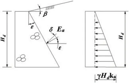
Figure 1:Gravity retaining wall with inclined infill top surface

2.2 Stability Analysis

2.2.1 Stress at Retaining Wall Base

The stress at the base of a retaining wall can be calculated in Eq.(3).

wherePmax/minis the maximum or minimum value of the retaining wall base stress(kPa);Gis the sum of vertical forces acting on the retaining wall(kN);∑Mis the sum of moments of all loads acting on the retaining wall with respect to the base centroid(kN·m);Ais the area of the base of the retaining wall(m2);andWis the elastic section modulus of the retaining wall base(m3).

The stresses of the retaining wall founded on hard rock should meet the following criteria:

(1) The maximum retaining wall base stress should not be greater than the allowable bearing capacity of the hard rock;and

(2) Except for the construction period and under an earthquake excitation, there must be no tensile stress on the base of the retaining wall.

2.2.2 Base Sliding Stability of Retaining Wall

The safety factor against sliding of the retaining wall along the rock base is calculated according to Eq.(4).

wheref′is the shear friction coefficient between the retaining wall and the rock base;c′is the adhesion between the retaining wall and the rock base(kPa);and ∑His the sum of the loads parallel to the base(kN).

When the retaining wall back surface is inclined towards the direction of the backfill,the safety factor along the surface between the retaining wall and rock can be calculated according to Eq.(5).

whereαis the angle between the base and a horizontal plane (°); andf0is the effective friction coefficient between the retaining wall and the soil that can be calculated in Eq.(6).

2.3 Overturning Stability

The factor of safety against overturning of a retaining wall is calculated according to Eq.(7).

whereK0is the overturning safety factor of the retaining wall;∑MVis the sum of clockwise moments with respect to the toe of the retaining wall(kN·m);and ∑MHis the sum counter-clockwise moments with respect to the toe of the retaining wall(kN·m).

According to the above formulas,the sliding stress is produced by the active earth pressure,and the resisting stresses include the compressive and shear strength at the wall base.However,the above results do not consider the tensile failure of the retaining wall.This paper presents a novel method of calculating the stresses and strains for a retaining wall.

3 New Landfill Analysis Method

When the shape of an object is determined,the stress solution must be clear and be updated with the boundary condition changes.Assuming the stresses are continuous, the solutions must satisfy the differential stress equilibrium equations and deformation boundary conditions.This method can be used to find the stress distribution for any geometry, including two-dimensional (2D) and three dimensional(3D) cases.When the boundary conditions and stress field are discontinuous,the discontinuous stress and displacement solutions can also be obtained.The landfill with a retaining wall is taken as an example to illustrate the basic ideas and approaches.

3.1 Boundary Conditions,Specific Gravity and Stresses

In this study,a theoretical solution for an arbitrary polygon under a 2D plane strain problem is studied.The landfill and the retaining wall are the polygon ABCDP and the quadrilateral element BCFE,respectively.The analysis steps are as follows:

(1)The boundaries of the analyzed system are assumed(see Fig.2).A linear equation is used for the boundary segments AB,BC,CD,DP,and PA of the polygon ABCDP,and segments BE,EF,FC,and CB of the quadrilateral BCFE.

(2) The specific gravity (γw,x,γw,y) distribution in the considered system is determined.In this context,γw,x=0 andγw,y=γ0is assumed for a landfill contained with a retaining wall.

(3) Using the stress field characteristics, the stress boundary conditions can be formed.The normal stresses at the transition between the landfill (i.e.,σnCD,fandσnDP,f) and the sliding bed(i.e.,σnCD,sandσnDP,s) are continuous, but the corresponding tangential stresses (i.e.,ττCD,f,ττDP,f,ττCD,s, andττDP,s) are not.The stresses between the landfill and retaining wall on plane BC (i.e.,σxx,σyy, andτxy)are continuous(see Fig.2).These assumptions can be written in Eqs.(8)and(9).

whereσnCD,f,σnDP,f,σnCD,s, andσnDP,sare the normal stresses of the landfill and the sliding bed planes CD and DP, respectively;σxxBC,f,σyyBC,f, andτxyBC,fare the stresses of the landfill on plane BC; andσxxBC,r,σyyBC,r, andτxyBC,rare the stresses of the retaining wall on plane BC.

(4) The landfill must satisfy the equilibrium equations, the stress boundary conditions, and the deformation equations.The expressions for the stress equilibrium equations are written and their coefficients are calculated.The stress expressions are assumed for a 2D landfill (note the stress expressions can be changed for different conditions)in Eqs.(10)–(12).

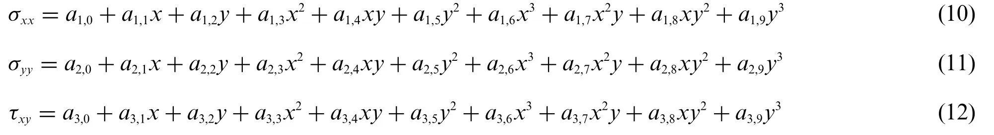
wherea1,i,a2,i,a3,i(i= 0, 1, 2, 3) are the coefficients;σxx,σyy, andτxyare X- and Y-direction normal stresses and shear stress,respectively.

The number of constant coefficients in Eqs.(10)–(12) can be reduced from 30 to 18 using the differential stress equilibrium equations,which depend on the boundary conditions and macro force equilibrium equations.

The following differential stress equilibrium equations, Eqs.(13) and (14), are satisfied at any point.

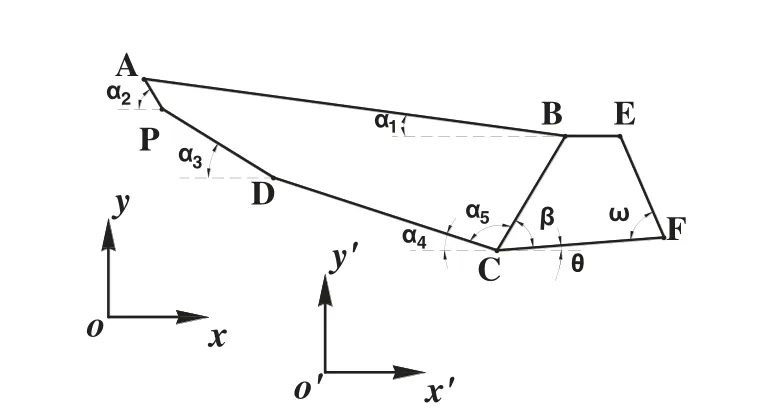
Figure 2:Sketch of landfill contained with retaining wall

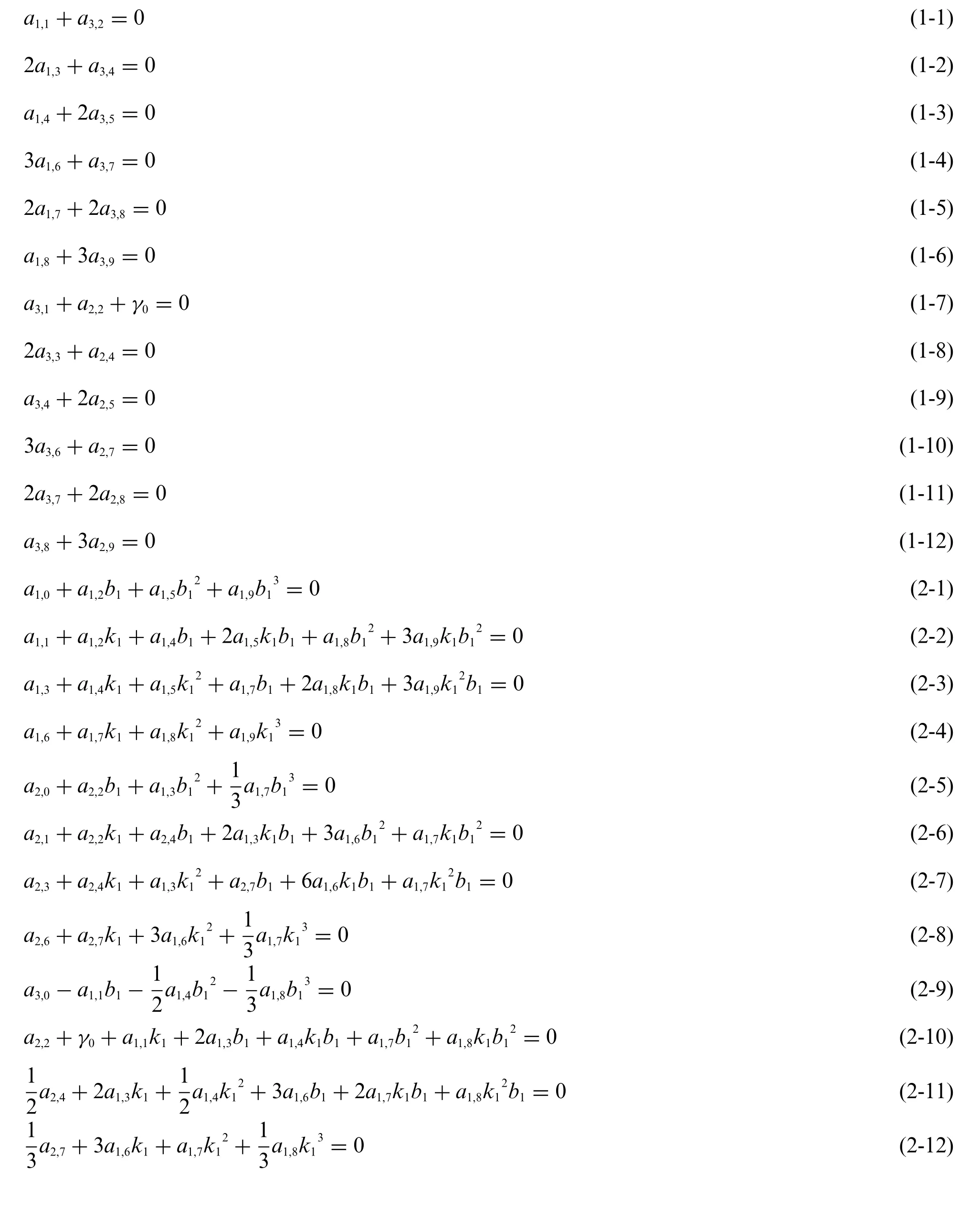
The corresponding coefficients are zero at any point with a constant unit weight(γ0≠0).This is a necessary condition for stress differential equilibrium equations.Eqs.(1-1)–(1-12)in Appendix are obtained using Eqs.(13)and(14).

3.2 Stress Relationships along Boundary Segment AB

Boundary segment AB of polygon ABCDP can be expressed mathematically in Eq.(15).

The stress conditions on boundary AB are in Eq.(16).

Eqs.(2-1)–(2-12)in Appendix were obtained using Eq.(16).

3.3 Force Equilibrium of Landfill

Once the landfill is in a balanced and stable state,the force equilibrium of polygon ABCDP in Xand Y-direction are in Eqs.(17)and(18).

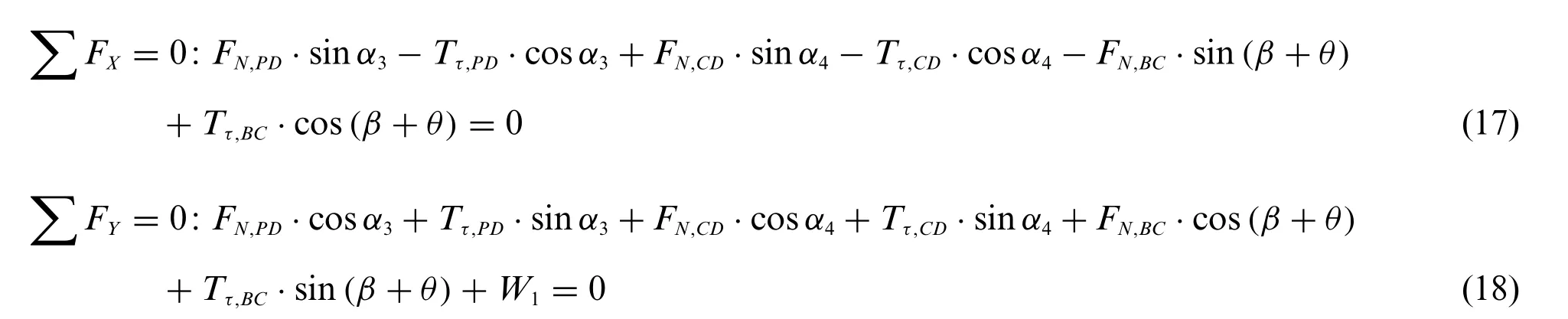
whereFN,PD,Tτ,PD,FN,CD,Tτ,CD,FN,BC, andTτ,BCare the normal and tangential forces on planes PD,CD,and BC,respectively;W1is the weight per unit thickness of polygon ABCDP;andα3,α3,α4,β, andθare the angles of different sides(see Fig.2).

The expressions forFN,PD,Tτ,PD,FN,CD,Tτ,CD,FN,BC,Tτ,BC, andW1are presented in the following sections.

3.3.1 Normal Forces Acting on Segments CD,BC,and PD

The equation of boundary segment CD is in Eq.(19)

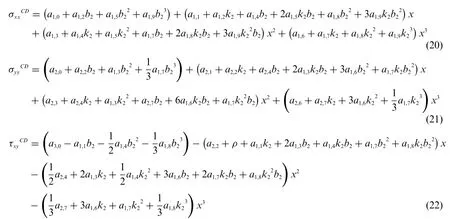
The expressions forσxxCD,σyyCD, andτxyCDare obtained by combining Eq.(19)and Eqs.(10)–(12),and are shown in Eqs.(20)–(22).

By substituting Eqs.(20)–(22)into the normal stress equations one obtains Eq.(23).

wherel1andm1are the directional cosines of segment CD given as follows:l1=cos(270°+α4),m1=cos(180°+α4)

The normal force acting on segment CD can be obtained by integration in Eq.(24).

The normal forces acting on segments BC and PD can be derived in a similar way.The equation for segment BC is in Eq.(25)and for PD is Eq.(26).

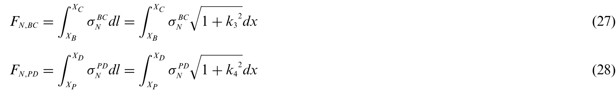
The resulting normal forces acting on segments BC and PD are in Eqs.(27)and(28),respectively.

3.3.2 Tangential Forces Acting on Segments CD and PD

The shear stresses between the landfill and the sliding bed are discontinuous.The frictional stresses along segment CD can be taken as the residual stress due to the sliding body with the landfill and expressed in Eq.(29).

where,c, andφare the normal stress,cohesion,and residual frictional for segment CD,respectively.The cohesion along segment CD can be taken as zero for unconsolidated waste.Therefore,Eq.(29)reduces to Eq.(30).

By integrating Eq.(30),we obtain Eq.(31).

Simplifying Eqs.(30)and(31)yields Eq.(32).

The equation for segment PD isy=k4x+b4,and the tangential force acting on segment of PD is given in Eq.(33).

3.3.3 Tangential Force Acting on Segment BC

The stresses between the landfill and the retaining wall are continuous.A similar method is adopted to calculate the shear stress along segment BC in Eq.(34), wherel2= cos(270°-β-θ)andm2=cos(360°-β-θ).

wherel2andm2are the directional cosines of segment BC.The resultant tangential force can be obtained by integrating Eq.(34)as in Eq.(35).

3.3.4 Weight of Polygon ABCDP

The weight(W1)can be calculated using the area(S1)of the sliding body in Eq.(36).

asW1=S1γ1,whereγ1is the unit weight of the sliding body(polygon ABCDP).

3.4 Stress along Segment AP

The equation of boundary segment AP is in Eq.(37).

The shear stress resultant along segment AP can be assumed zero according to the Saint Venant principle shown in Eq.(38).

3.5 Coefficients for Landfill Solution

If coefficientsa1,0,a2,0, anda3,0are assumed to be zero,their total number is reduced to 15 by using Eqs.(1-1)–(1-12)in Appendix.The 15 coefficients(a1,1,a1,2,a1,3,a1,4,a1,5,a1,6,a1,7,a1,8,a1,9,a2,1,a2,2,a2,3,a2,4,a2,6, anda2,7) can be obtained using Eqs.(2-1)–(2-12) in Appendix and Eqs.(17), (18), and (38).The stress solution coefficients are calculated by using the expressions forσxx,σyy, andτxy.

4 Theoretical Solution for Retaining Wall

The stresses acting on segments BC and CF of the retaining wall have been obtained.This section derives the stresses for the retaining wall assuming stress continuity between the landfill and the retaining wall.The coordinates used to analyze the retaining wall are shown Fig.3.

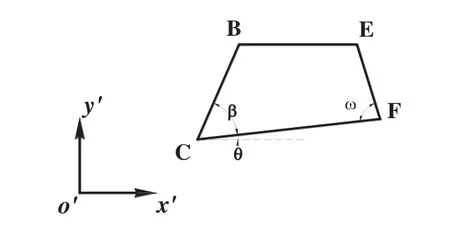
Figure 3:2D model of retaining wall

4.1 Stress Continuity along Boundary Segment BC

Stress equilibrium is assumed along segments BC and CF based on the continuity of stresses between the landfill and the retaining wall and between the retaining wall and its base.

The equation for segment BC is Eq.(39).

In Eq.(40),x′andy′are the new coordinates,andX1andY1are the coordinates of the origin of the new coordinate system with respect to the old coordinate system.

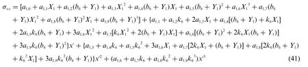
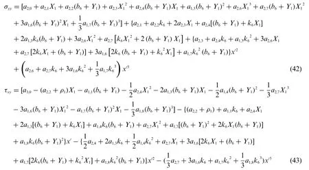
By combining Eqs.(39) and (40) with Eqs.(10)–(12), the normal and tangential stresses are calculated in Eqs.(41)–(43).

The stresses acting on the retaining wall are defined in thex′o′y′coordinate system in Eqs.(44)–(46).

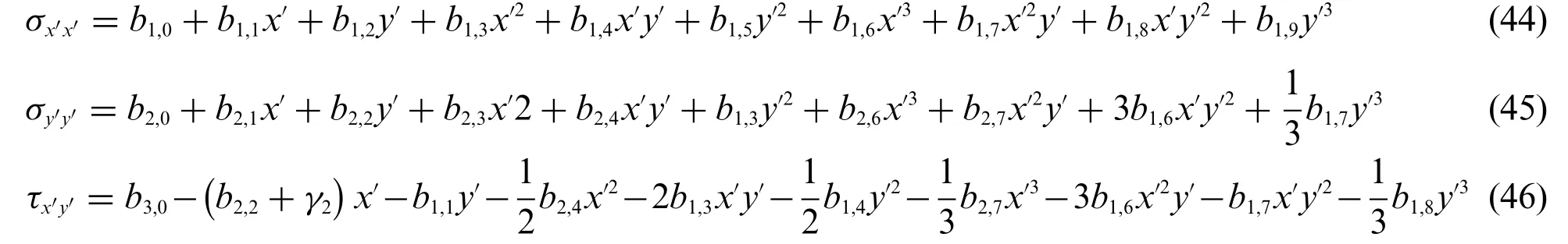
whereb1,i,b2,i, andb3,i(i=0,1,...,9)are the constant coefficients;σx′x′,σy′y′, andτx′y′are the stresses along x’- and y’- directions and the shear stress, respectively; andγ2is the specific weight of the retaining wall.

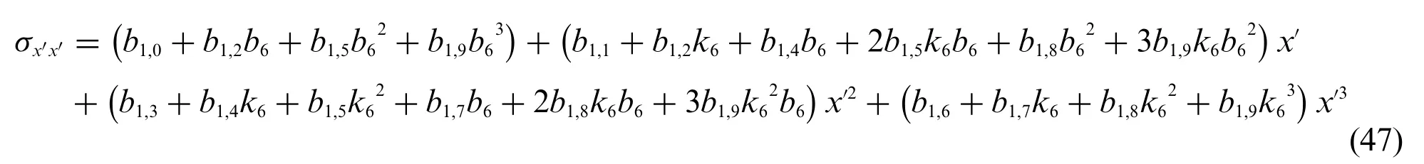
Eq.(39)is substituted into Eq.(44)to yield Eq.(47).

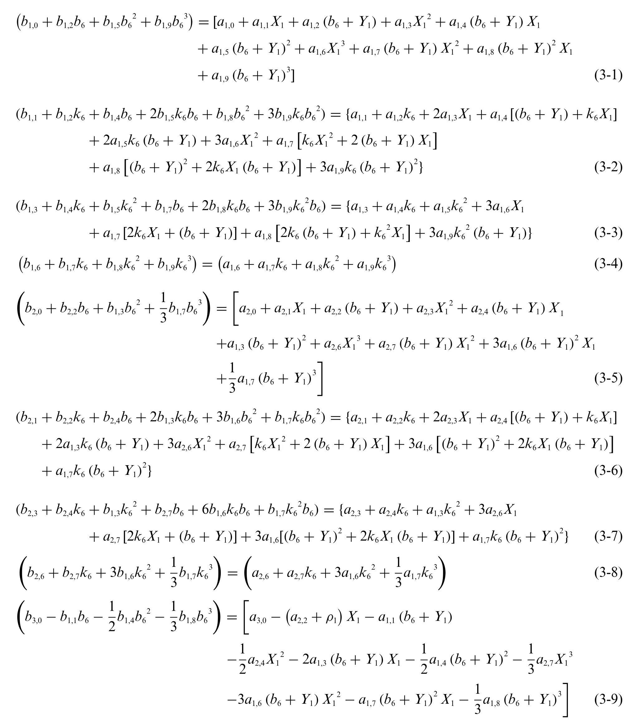
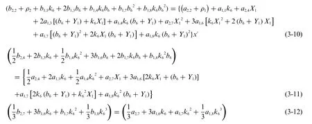
Eqs.(3-1)–(3-4)in Appendix can be obtained assumingσx′x′=-σxxand using Eqs.(41)–(47).The same method is used assumingσy′y′=-σyyandτx′y′=-τxyto obtain Eqs.(3-5)–(3-12)in Appendix.

4.2 Force Balance of Retaining Wall

The forces acting on the retaining wall include the normal and tangential forces along segment BC(and)and segment CF(and),and weight(W2)(see Fig.4).The force equilibrium in thex′-andy′-directions must be satisfied.

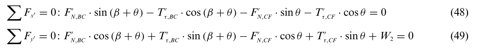
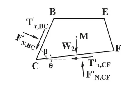
Figure 4:Force acting on retaining wall

The calculation statements are presented in the following form:

4.2.1 Normal Forces along Segments BC and CF

Eq.(50)for the retaining wall can be obtained using Eqs.(44)–(46).

wherel4andm4are the directional cosines of segment BC of the retaining wall,and

l4=cos(270°-β-θ),m4=cos(360°-β-θ)

The normal force acting on boundary segment BC of the retaining wall is obtained by integrating Eq.(51).

The normal stress on boundary segment CF is in Eq.(52).

In Eq.(53),l5andm5are the directional cosines of segment CF of the retaining wall, andl5=cos(270°-θ),m5=cos(360°-θ).

The normal force acting on boundary segment CF of the retaining wall is obtained by integrating Eq.(53),as shown in Eq.(54).

4.2.2 Tangential Forces along Segments BC and CF

A similar approach is adopted for calculating the tangential forces along segments BC and CF of the retaining wall in Eq.(55).

The tangential force acting on boundary segment BC can be achieved by integrating Eq.(55)in Eq.(56).

The shear stress acting on segment CF is in Eq.(57).

The tangential force acting on boundary segment CF is found by integrating Eq.(57)as shown in Eq.(58).

4.2.3 Weight and Barycentric Coordinate of Retaining Wall

The barycentric coordinates of triangles BEC and EFC are denoted as I and J,respectively.The barycent ric coordinatesof trapezoid BCFE can be obtained and the weight(W2)can be calculated using the area(S2)of the retaining wall,shown in Eq.(59)and Fig.5.

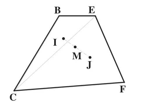
Figure 5:Retaining wall barycentric coordinate determination

The weight per unit thickness of the retaining wall isW2=S2γ2.The moment of weight per unit thickness(MW2)of the retaining wall isis the point with respect to which the moment is calculated.

4.3 Moment Balance of Retaining Wall

MomentsMW2,MBG,MCG,MBC,MCP,MPF, andMCF,shown in Fig.6,can be obtained.

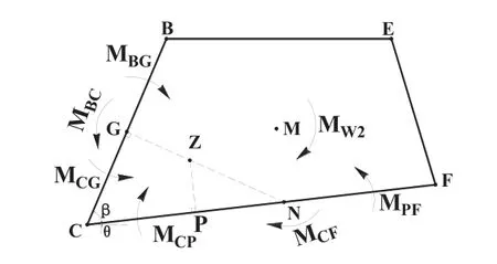
Figure 6:Moments acting on retaining wall

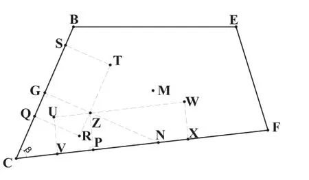
Figure 7:Lever arms of moment acting on retaining wall

The moment balance equation for the retaining wall can be written in Eq.(62).

The lever arms of momentsMW2,MBG,MCG,MBC,MCP,MPF, andMCFare shown in Fig.7.The detailed formulas for the moments are shown in Eqs.(4-1)–(4-7)in Appendix.

4.4 Free Point Stress Characteristics

σx′x′|E=0,σy′y′|E=0,τx′y′|E=0

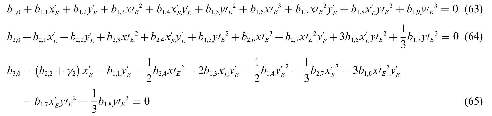
Therefore,we have Eqs.(63)–(65).

4.5 Coefficients of Retaining Wall Solution

The 18 coefficientsb1,0,b1,1,b1,2,b1,3,b1,4,b1,5,b1,6,b1,7,b1,8,b1,9,b2,0,b2,1,b2,2,b2,3,b2,4,b2,6,b2,7, andb3,0are obtained by using Eqs.(3-1)–(3-12) in Appendix, two force equilibrium equations (Eqs.(48)and(49)),the moment equilibrium equation(Eq.(62)),and there stress equations at stress-free point E (Eqs.(63)–(65)).The stresses at each point on the retaining wall can be determined from the expressions forσx′x′,σy′y′, andτx′y′.

5 Strain Field in Landfill with Retaining Wall

5.1 Strain Distribution in Landfill

The Duncan-Chang constitutive model is employed to describe the strain distribution in the landfill.The basic equations are Eqs.(66)and(67).

whereσ1andσ3are the maximum and minimum principal stresses,respectively;ε1andε3are the strains in the direction of maximum and minimum principal stresses, respectively; anda1,b1,a2, andb2are coefficients.

The expressions for strains(εij)in different directions for a 2D problem can be written as Eqs.(68)–(70).

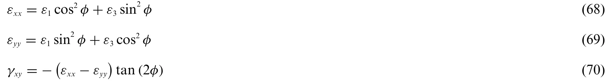
whereεxx,εyy, andγxyare the strain components;andφis the rotation angle.The angle of rotation(φ)is measured relative to the minimum principal stress(σ3)direction and can be expressed in Eqs.(71)and(72).

5.2 Strain Distribution in Retaining Wall

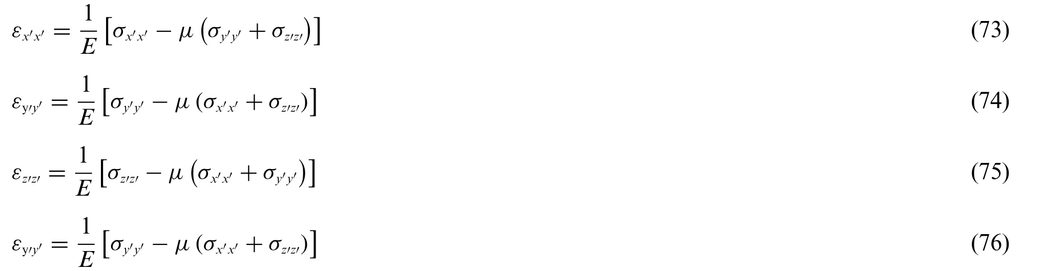
The retaining wall can be assumed to be a plane strain problem, i.e.,εz′= 0 andσz′≠ 0.The general Hooke law gives Eqs.(73)–(76).

6 Case Study

6.1 Overview of Case Study Landfill Project

A case study of a landfill project located in Fengjiadagou of Guandukou Town of Badong County in Hubei Province of China is studied.The national road No.209 passes to the west side of the landfill.The landfill area is about 2.1×104m2and the effective waste storage capacity of the landfill is 10.5×104m3.The daily average processing capacity of the landfill is 230 kN/d for 5 years.Currently,the landfill is closed(see Fig.8).

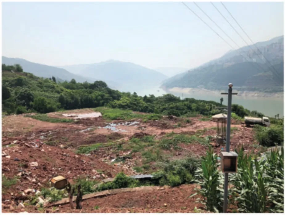
Figure 8:Current condition of Guandukou Town landfill

The elevation of the landfill back side is 262 m and the elevation of its front side at the top surface of the retaining wall is 225 m.The sloped length of the landfill is about 54.3 m and its width is 37 m with a slope angle of about 20° (see Figs.9 and 10).The original top layer of the landfill comprises residual soil and strongly weathered red sandstone,which has been removed(see Figs.9 and 10).The sandstone (T2b2) has a high uniaxial compressive strength of 40 MPa to 60 MPa.The dip angle of the sandstone layer is 26°to 30°,and the foundation of the retaining wall is located on a moderately weathered sandstone(see Fig.10).

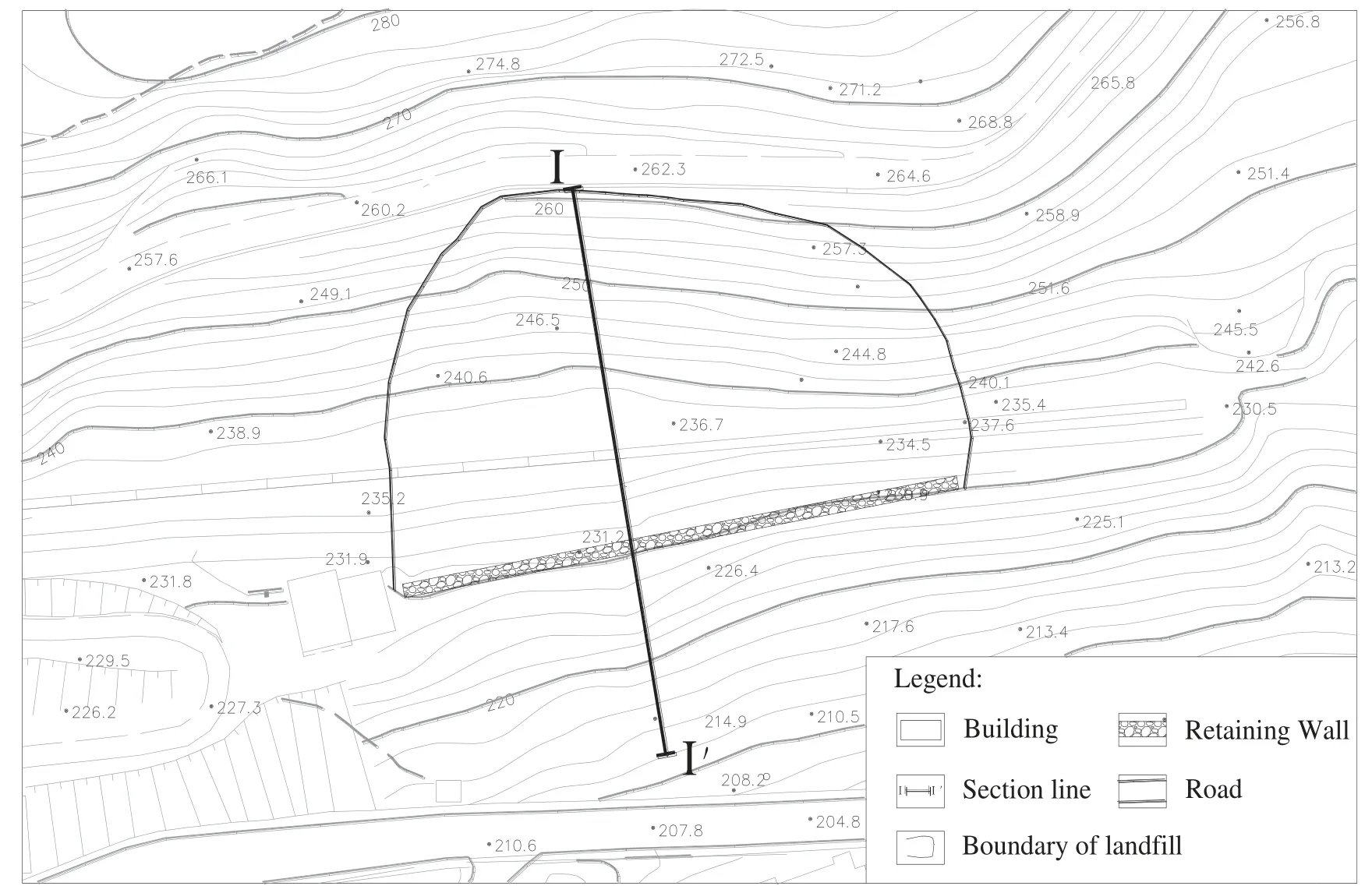
Figure 9:Landfill area layout

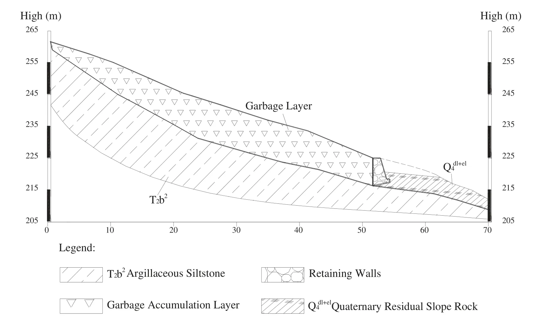
Figure 10:Section I-I of landfill

6.2 Calculations

6.2.1 Analytical Model

The analytical model was established according to profile I-I of the Guandukou Town landfill(see Fig.2).The unit weight of the waste was taken as 19 kN/m3,and the residual frictional angle between the waste and rock surface as 9°.The method described in this paper was used to obtain the stress and strain fields in the landfill and the retaining wall.

The dimensions and angles of the landfill ABCDP are as follows:AB=54.3 m,AP=1.3 m,PD=26.9 m,DC=28.8 m,BC=4.3 m,α1=20°,α2=77°,α3=31°,α4=15°,andα5=74°.

The dimensions and angles of the retaining wall are as follows:EB=1.2 m,BC=4.3 m,CF=2.4 m,FE=4.1 m andβ=79°,θ=12°,andω=85°.

6.2.2 Stress and Strain Fields in Landfill

Eighteen coefficients were determined for the landfill solutions under the condition that the force boundary conditions and stress differential equilibrium equations are satisfied.Their values for the stress field(see Fig.11c)are as follows:

a1,0=0kPa,a1,1=19.61kPa/m,a1,2=-232.23kPa/m,a1,3=3.02kPa/m2,a1,4=-4.91kPa/m2,a1,5=31.02kPa/m2,

a1,6= -0.02kPa/m3,a1,7= -0.17kPa/m3,a1,8= 0.23kPa/m3,a1,9= -1.04kPa/m3,a2,1=-12.54kPa/m,

a2,2= -32.79kPa/m,a2,3= 0.16kPa/m2,a2,4= 1.74kPa/m2,a2,6= -0.0005kPa/m3,a2,7=-0.01kPa/m3.

The parameters of the Duncan-Chang constitutive model are as follows:a1= 0.0002,a2=0.00012099,b1= –0.000056, andb2= 0.0002099 (see Eqs.(66) and (67)).These parameters were obtained using the experimental principal strains of the landfill that are presented in Figs.12a and 12b and the strain fields shown in Figs.13a–13c.

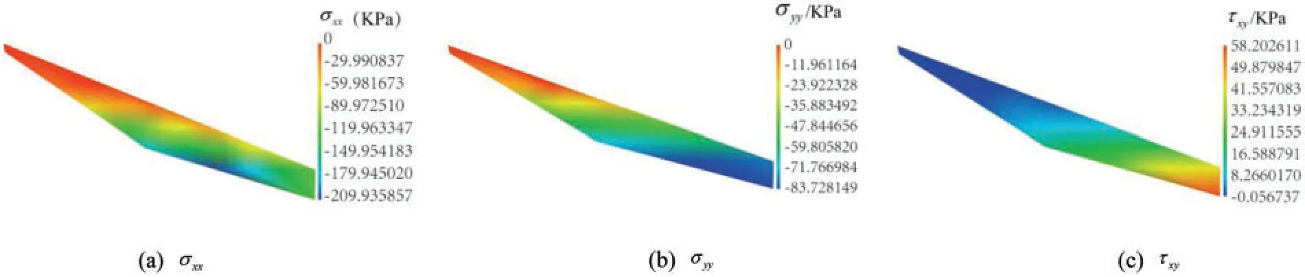
Figure 11:Distributions of stresses σxx,σyy,and τxy in landfill

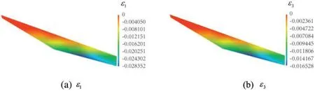
Figure 12:Distributions of principal strains ε1 and ε3 in landfill

Figure 13:Distributions of strains εxx,εyy,and γxy in landfill

6.2.3 Retaining Wall Analysis

The unit weight of the retaining wall was assumed as 25 kN/m3,the elastic modulus asE=300 MPa,and the Poisson ratio asμ=0.11,respectively.The 18 coefficients of the retaining wall solution were obtained under the conditions that the stresses on the boundaries and equilibrium equations are satisfied as follows:

b1,0= -126.67kPa,b1,1= 188.00kPa/m,b1,2= -291.99kPa/m,b1,3= -10.44kPa/m2,b1,4=-6.50kPa/m2,

b1,5= 33.38kPa/m2,b1,6= 0.42kPa/m3,b1,7= -0.21kPa/m3,b1,8= 0.23kPa/m3,b1,9=-1.04kPa/m3,

b2,0=669939.82kPa,b2,1=-175637.48kPa/m,b2,2=-2913.50kPa/m,b2,3=15155.09kPa/m2,b2,4=625.17kPa/m2,b2,6=-429.55kPa/m3,b2,7=-33.14kPa/m3,b3,0=-8516.71kPa.

The stress and principle stress fields in the retaining wall are presented in Figs.14a–14e.If the peak stress in the retaining wall meets the Mohr-Coulomb criterion and the friction angle is taken asφ=40°,the corresponding cohesion(C)distribution in the retaining wall is as shown in Fig.14f.The strain fields in the retaining wall are presented in Figs.15a–15c.

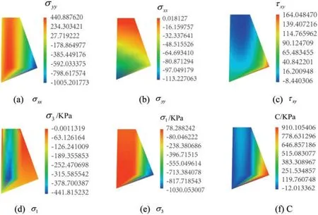
Figure 14:Distributions of stresses σxx,σyy,τxy,σ1,and σ3,and values of C in retaining wall

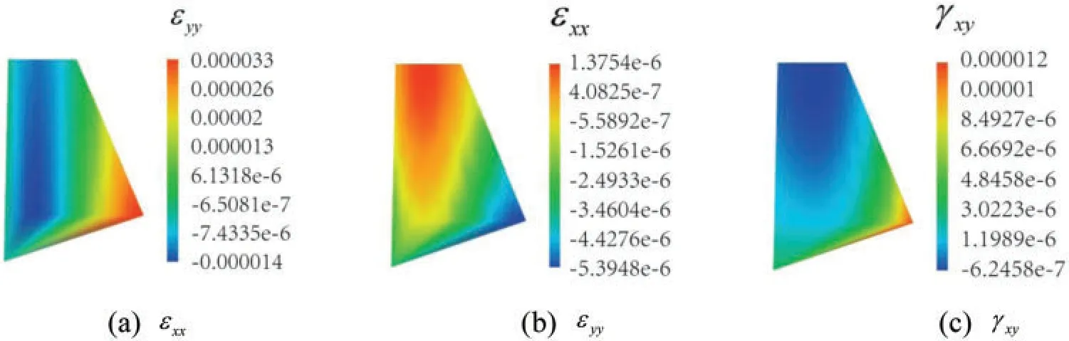
Figure 15:Distributions of strains εxx,εyy,and γxy in retaining wall

6.2.4 Analysis of Results for Landfill with Retaining Wall

Landfill Stress and Strain Field Characteristics

The obtained stress and strain fields in the landfill are logical.Stressesσxxandσyyare compressive stresses,and the local tensile shear stresses(τxy)exist,especially at the toe of the landfill.These stress and strain fields are consistent with the actual stresses observedin situ.

Strength Distribution Characteristics in Retaining Wall

The conventional factor of safety against sliding(i.e.,Kc= 1.563)along the rock bed at the base and that against overturning(i.e.,K0=1.615)of the retaining wall were obtained by assumingf0=1.5 andc0=1200 kPa in Eqs.(4)and(7),respectively,These safety factors meet the design requirements.

From the results of the proposed method,it can be seen that the maximum tensile stress is located at point B (78.2 kPa).This value is lower than the strength of M15 mortar and block stone used in the project.The maximum compressive stress (1005 kPa) is located at point F of the retaining wall,which is less than the strength of the retaining wall material.At any point in the retaining wall, the cohesion intercept(C)value is less than 910 kPa(see Fig.14f)for the internal friction angle of 40°.The cohesion is within the mortar and the block stone acceptable values, thus the shear failure does not occur at any point on the retaining wall.At the interface between the retaining wall and its foundation,the maximum compressive,shear,and tensile stresses are all less than the corresponding strengths.

The ANSYS finite element software was also employed to study the stresses and strains within the landfill and the retaining wall(see Fig.16).The normal displacement constraints along boundary segments CF, CD, and DP were applied.The differences between the results of the finite element model and the method proposed in this paper were less than 15% for the landfill and 7% for the retaining wall,respectively.The factors of safety for stability along the interface between the retaining wall and its base were also determined and found to differ by more than 5%(see Fig.17).Note thatis the factor of safety of the slope calculated along segment CF,calculated as(=C+tanφ,andCandφare the cohesion and frictional angle of the interface between the retaining wall and the base,respectively).S3is the distance from point C to point F(m).The factors of safety satisfy the requirements of the retaining wall stability.

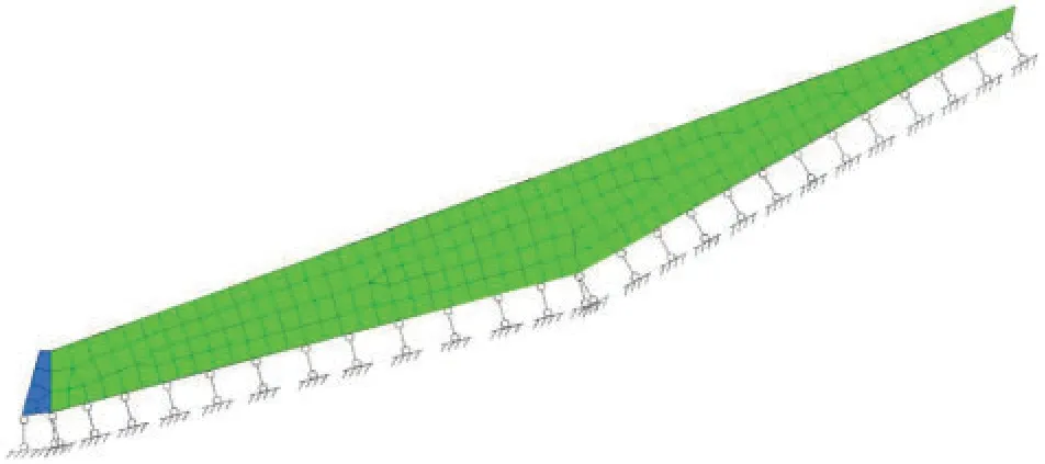
Figure 16:FEM of landfill with retaining wall

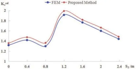
Figure 17:Factor of safety at the interface of retaining wall and base

Based on the traditional analysis of the retaining wall(the limited rigid body balance method and FEM)and the proposed methods in this paper,the studied retaining wall is in a stable condition.

7 Conclusions

(1) The stress and strain field characteristics of the landfill and the retaining wall have been determined.The following conclusions can be drawn:The stress fields in the landfill and the retaining wall are non-linear within the domain.The analytical method proposed in this article can provide a theoretical basis for the control design and displacement prediction of a slope and a retaining wall.Based on the geometry and material of the retaining wall,novel methods for preventing retaining wall failures can be proposed and validated.

(2) The analytical solutions presented in this article are based on the assumption that the stresses are continuous or discontinuous.It is acceptable that the results of the proposed method in this paper are comparable to that of the finite element method under the given boundary conditions.

(3) In this article, the limit equilibrium state hypothesis was ignored for the retaining wall.The stresses acting on the retaining wall included normal stress and the shear stress.

(4) The design methodology of the retaining wall was explained using the results of the numerical analysis.According to the analytical results,the tensile and bulging failure characteristics of the retaining wall and the landfill can be determined.The internal failure of the retaining wall and the landfill can be conducted at any point within the domain,and therefore a new stability analysis method for the anti-sliding design was proposed.

Appendix

The moment analysis is presented below;for force lever arms see Fig.7.

Segment BC:

Any point Q is chosen,X’coordinate is between X’Cand X’G,and the lever arm ofσnisand thenThe equation of line BC isy′=k6x′+b6,then:

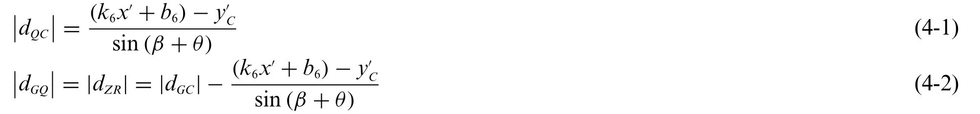
Any point S is chosen,X’coordinate is between X’Gand X’B,and the lever arm ofσnis

|dGS|=|dTZ|.The equations of lines BC and GN arey′=k6x′+b6andy′=k8x′+b8,respectively.Then:

The lever arm ofτnis|dGZ|for the whole segment BC.

Segment CF:

(1)Any point V is chosen,X’coordinate is between X’Cand X’P,and the lever arm ofσnis

|dUZ|=|dVP|,and|dVP|=|dCP|-|dCV|.

The equation of straight line CF isy′=k7x′+b7,then:

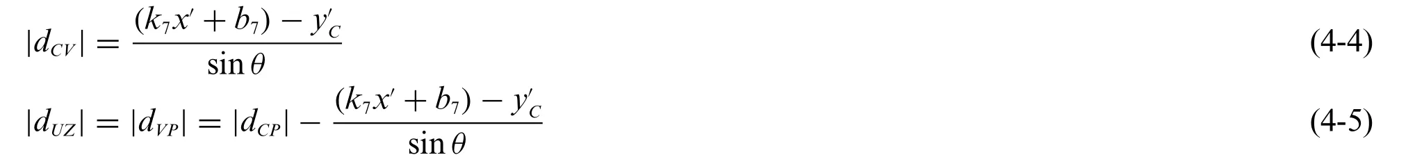
(2)Any point X is chosen,X’coordinate is between X’Pand X’F,and the lever arm ofσnis|dZW|=|dPX|.

The equation of straight line CF isy′=k7x′+b7,and

The lever arm ofτnis|dZP|for the entire segment CF,and ∑MZ=0:

Funding Statement:This work was supported by the National Key R&D Program(No.2018YFC1504901), and by the Natural Science Foundation of China (Grant No.42071264).This work was also supported by the Geological Hazard Prevention Project in The Three Gorges Reservoirs(Grant No.0001212015CC60005).

Conflicts of Interest:The authors declare that they have no conflicts of interest to report regarding the present study.