LaNets:Hybrid Lagrange Neural Networks for Solving Partial Differential Equations

Ying Li,Longxiang Xu,Fangjun Mei and Shihui Ying

1School of Computer Engineering and Science,Shanghai University,Shanghai,200444,China

2School of Science,Shanghai University,Shanghai,200444,China

ABSTRACT We propose new hybrid Lagrange neural networks called LaNets to predict the numerical solutions of partial differential equations.That is, we embed Lagrange interpolation and small sample learning into deep neural network frameworks.Concretely,we first perform Lagrange interpolation in front of the deep feedforward neural network.The Lagrange basis function has a neat structure and a strong expression ability, which is suitable to be a preprocessing tool for pre-fitting and feature extraction.Second, we introduce small sample learning into training,which is beneficial to guide the model to be corrected quickly.Taking advantages of the theoretical support of traditional numerical method and the efficient allocation of modern machine learning,LaNets achieve higher predictive accuracy compared to the state-of-the-art work.The stability and accuracy of the proposed algorithm are demonstrated through a series of classical numerical examples,including one-dimensional Burgers equation,onedimensional carburizing diffusion equations,two-dimensional Helmholtz equation and two-dimensional Burgers equation.Experimental results validate the robustness,effectiveness and flexibility of the proposed algorithm.

KEYWORDS Hybrid Lagrange neural networks; interpolation polynomials; deep learning; numerical simulation; partial differential equations

1 Introduction

In this paper,we consider partial differential equations(PDEs)of the general form in Eqs.(1.1)–(1.3):

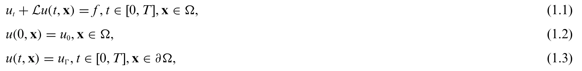
whereLis a differential operator,Ωis a subset of RN, and∂Ωrepresents its boundary.udenotes the unknown function that needs to be solved,u0anduΓrepresent initial and boundary conditions,respectively.Different governing equations and homologous initial/boundary conditions can describe many physical phenomena in nature, but it is practically difficult to find the analytical solutions.Therefore,more and more scholars have tried a variety of numerical methods to solve PDEs in recent years.

At first,traditional numerical methods,including finite element method[1],finite volume method[2] and finite difference method [3], were usually used to solve partial differential equations.Afterwards, with the rapid development of machine learning [4–6], the universal approximation ability of neural networks is considered to be helpful for obtaining approximated solutions of differential equations.Han et al.[7–9] proposed deep learning-based numerical approaches to solve variational problems, backward stochastic differential equations and high-dimensional equations.Then Chen et al.[10] extended their work to solve Navier-Stokes and Cahn-Hillard equation.Sirignano et al.[11] combined Galerkin method and deep learning to solve high-dimensional free boundary PDEs.Raissi et al.[12] proposed the physics-informed neural network (PINNs) framework which acts as the benchmark algorithm in this field.In PINNs, physical constraints are added to limit the space of solutions to improve the accuracy.Futhermore,many scholars carry out research based on this method.Dwivedi et al.[13] incorporated PINNs with extreme learning machine to solve timedependent linear partial differential equations.Pang et al.[14]solved space-time fractional advectiondiffusion equations by expanding PINNs to fractional PINNs.Raissi et al.[15]subsequently developed a physics-informed deep learning framework that is able to encode Navier-Stokes equations into the neural networks.Kharazmi et al.[16] constructed a variational physics-informed neural network to effectively reduce the training cost in network training.Yang et al.[17] proposed Bayesian physicsinformed neural networks for solving forward and inverse nonlinear problems with PDEs and noisy data.Meng et al.[18]developed a parareal physics-informed neural network to significantly accelerate the long-time integration of partial differential equations.Gao et al.[19] proposed a new learning architecture of physics-constrained convolutional neural network to learn the solutions to parametric PDEs on irregular domains.

Neural network is a black box model,its approximation ability depends partly on the depth and width of the network,and thus too many parameters will cause a decrease in computational efficiency.One may use Functional Link Artificial Neural Network (FLANN) [20] model to overcome this problem.In FLANN, the single hidden layer of neural network is replaced by an expansion layer based on distinct polynomials.Mall et al.[21]used Chebyshev neural network to solve elliptic partial differential equations by replacing the single hidden layer of the neural network with Chebyshev polynomials.Sun et al.[22] replaced the hidden layer with Bernstein polynomials to obtain the numerical solution of PDEs as well.Due to the application of polynomials, neural network has no actual hidden layers,and the number of parameters is greatly reduced.

On the other hand,deep learning is a type of learning that requires a lot of data.The performance of deep learning depends on large-scale and high-quality sample sets but the cost of data acquisition is prohibitive.Moreover,sample labeling also needs to consume a lot of human and material resources.Therefore, a popular learning paradigm named Small Sample Learning (SSL) [23] has been used in some new fields.SSL refers to the ability to learn and generalize under a small number of samples.At present,SSL has been successfully applied in medical image analysis[24],long tail distribution target detection[25],remote sensing scene classification[26],etc.

In this paper, we integrate Lagrange interpolation and small sample learning with deep neural networks frameworks to deal with the problems in existing models.Specifically, we replace the first hidden layer of the deep neural network with a Lagrange block.Here, Lagrange block is a preprocessing tool for preliminary fitting and feature extraction of input data.The Lagrange basis function has a neat structure and strong expressive ability, so it is fully capable of better extracting detailed features of input data for feature enhancement.The main thought of Lagrange interpolation is to interpolate the function values of other positions between nodes through the given nodes,so as to make a prefitting behaviour without adding any extra parameters.Then, the enhanced vector is input to the subsequent hidden layer for the training of the network model.Furthermore,we add the residual of a handful of observations into cost function to rectify the model and improve the predictive accuracy with less label data.This composite neural network structure is quite flexible,mainly in that the structure is easy to modify.That is,the number of polynomials and hidden layers can be adjusted according to the complexity of different problems.

The structure of this paper is as follows.In Section 2, we present the introduction of Lagrange polynomials,the structure of the LaNets and the steps of algorithm.Numerical experiments for onedimensional PDEs and two-dimensional PDEs are described in Section 3.Finally, conclusions are incorporated into Section 4.

2 LaNets:Theory,Architecture,Algorithm

In this section,we start with illustrations on Lagrange interplotation polymonials.After that,we discuss the framework of LaNets.And finally,we clarify the detatils of the proposed algorithm.

2.1 Lagrange Interpolation Polynomial

Lagrange interpolation is a kind of polynomial interpolation methods proposed by Joseph-Louis Lagrange,a French mathematician in the 18th century,for numerical analysis[27].Interpolation is an important method for the approximation of functions,which uses the value of a function at a finite point to estimate the approximation of the function at other points.That is,the continuous function is interpolated on the basis of discrete data to make the continuous curve pass through all the given discrete data points.Mathematically speaking,Lagrange interpolation can give a polynomial function that passes through several known points on a two-dimensional plane.

Assumingx1,x2,...,xn+1are the distinctn+1 points in the complex panels, andy1,y2,...,yn+1are the corresponding values atx1,x2,...,xn+1.The Lagrange polynomialL(x)corresponding to their degree not exceedingnis unique.Indeed,the uniqueness ofL(x)arises from the fact that the difference of two such polynomials vanish at pointsx1,...,xn+1without a degree greater thann.The following polynomial clearly possesses all the necessary properties in Eqs.(2)–(3):

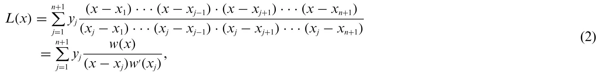
where

Here,the polynomialL(x)is called Lagrange interpolation polynomial.And the distinct pointsx1,...,xn+1are called the interpolation points.It can be seen that the corresponding Lagrange polynomial can be obtained by givenn+1 value points:(x0,y0),...,(xn,yn).The Lagrange interpolation polynomial obtained from only some points can replace the function to obtain the solution at any other points.The correctness of Lagrange polynomials has been proved in the literatures[27,28].

2.2 The Architecture of LaNets

Fig.1 displays the structure of LaNets, which is composed of two main parts.One is a preprocessing part based on Lagrange polynomials, the other is the training of deep feedforward neural network.Thus, the LaNets model we designed is a joint feedforward neural network composed of input layer,Lagrange block,hidden layers and output layer.As described in Section 2.1,we can also write Lagrange interpolation polynomial in Eq.(4):

wherexjandyjin the above formula correspond to the position of the independent variable and the value of function at this position, respectively.Here, we calllj(x)the Lagrange interpolation basis function,and the expression oflj(x)is as follows:

Figure 1:The schematic drawing of the LaNets

As shown in Fig.1,the original input vector is extended to a new enhanced vector by Lagrange block primarily,and then sent to deep feedforward neural network for training.The black Lagrange block on the right shows the Lagrange interpolation basis functionsl0,l1andl2visually.Spatiotemporal variables can be both handled with Lagrange basis functions.Actually,the proposed model not only increases the reliability and stability of the single-layer polynomial neural network,but also improves the predictive accuracy of the deep feedforward neural network without adding any extra parameters.

2.3 Loss Function&Algorithm

The problem we aim to solve is described as Eqs.(1.1)–(1.3).Following the original work of Raissi et al.[12],F(t,x)can be defined as Eq.(6):

We continue to approximateu(t,x)with the deep neural networku(t,x;θ),where θ represents the parameter set of the network.The model is then trained by minimizing the following compound loss functionJ(θ)in Eq.(7):

An entire overview of this work is shown in Algorithm 1.In the algorithm description,we consider the spatio-temporal variables x andt.Without a doubt,the proposed method is also applicable to timeindependent partial differential equations, and related examples will be mentioned in the following experiments.

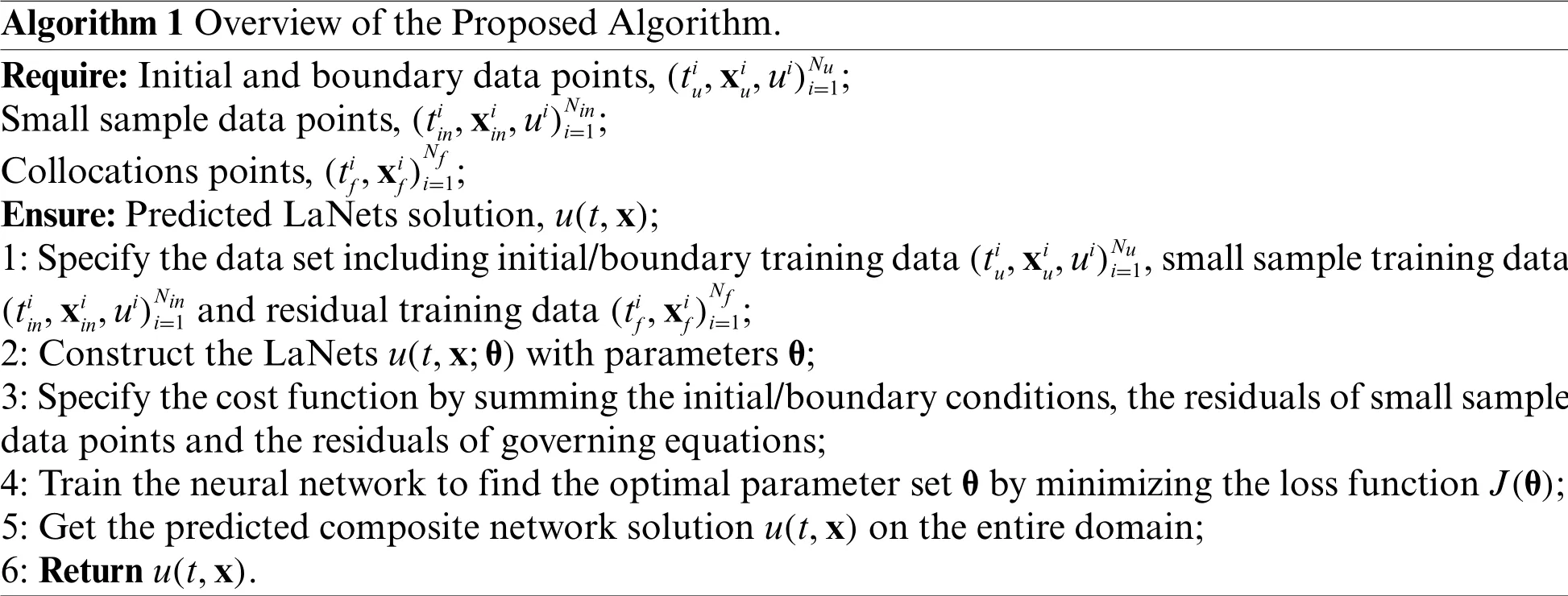
Algorithm 1 Overview of the Proposed Algorithm.Require:Initial and boundary data points,(tiu,xiu,ui)Nu i=1;Small sample data points,(ti in,ui)Nin i=1;Collocations points,(ti in,xi f,xi f)Nf i=1;Ensure:Predicted LaNets solution,u(t,x);1:Specify the data set including initial/boundary training data(tiu,xiu,ui)Nu i=1,small sample training data(ti in,xiin,ui)Nin i=1 and residual training data(ti f,xi f)Nf i=1;2:Construct the LaNets u(t,x;θ)with parameters θ;3:Specify the cost function by summing the initial/boundary conditions,the residuals of small sample data points and the residuals of governing equations;4:Train the neural network to find the optimal parameter set θ by minimizing the loss function J(θ);5:Get the predicted composite network solution u(t,x)on the entire domain;6:Return u(t,x).

3 Numerical Experiments

In this section, we verify the performance and accuracy of LaNets numerically through experiments with benchmark equations.In Subsection 3.1,we provide three typical one-dimensional timedependent PDEs to validate the robustness and validity of the proposed algorithm.In Subsection 3.2,two-dimensional PDEs are shown to illustrate the reliability and stability of the method.

3.1 Numerical Results for One-Dimensional Equations

In this subsection, we demonstrate the predictive accuracy of our method on three onedimensional time-dependent PDEs including Burgers equation, carburizing constant diffusion coefficient equation and carburizing variable diffusion coefficient equation.

3.1.1 Burgers Equation

We start with the following one-dimensional time-dependent Burgers equation in Eqs.(8.1)–(8.3):

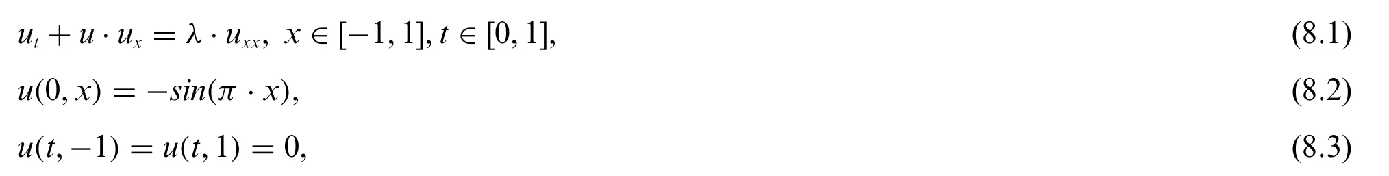
whereλis the viscosity parameter.In this case,we takeλ=0.01/π.

Here,the LaNets model consists of one Lagrange block and 7 hidden layers with 20 neurons in each layer.Lagrange block contains three Lagrange basis functions.By default,the Lagrange block is composed of three Lagrange basis functions unless otherwise specified.Fig.2a illustrates the predicted numerical result of the Burgers equation,and the relativeL2error measured at the end is 3.84×10-4.The loss curvevs.iteration is displayed in Fig.2b.The mean square error loss decreases steadily,which illustrates the stability of the proposed method.

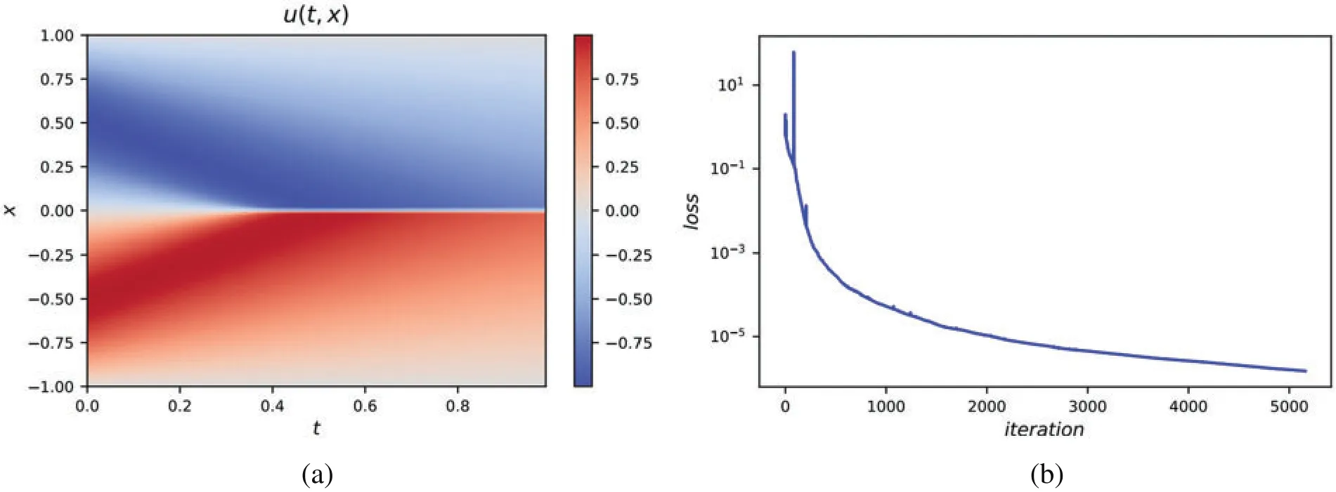
Figure 2:(a) The predicted solution of one-dimensional Burgers equation.Here, we adopt a 9-layer LaNets.The size of small sample points is 100.The relative L2 error measured is 3.84×10-4.(b)The loss curve vs.iteration

To further verify the effectiveness of the proposed algorithm,we compare the predicted solution with the analytical solution provided in the literature[30]at four timesnapshots,which are presented in Fig.3.It seems that there is almost no difference between the predicted solution and the exact solution.Moreover,the sharp gap formed near timet=0.65 is also well captured.

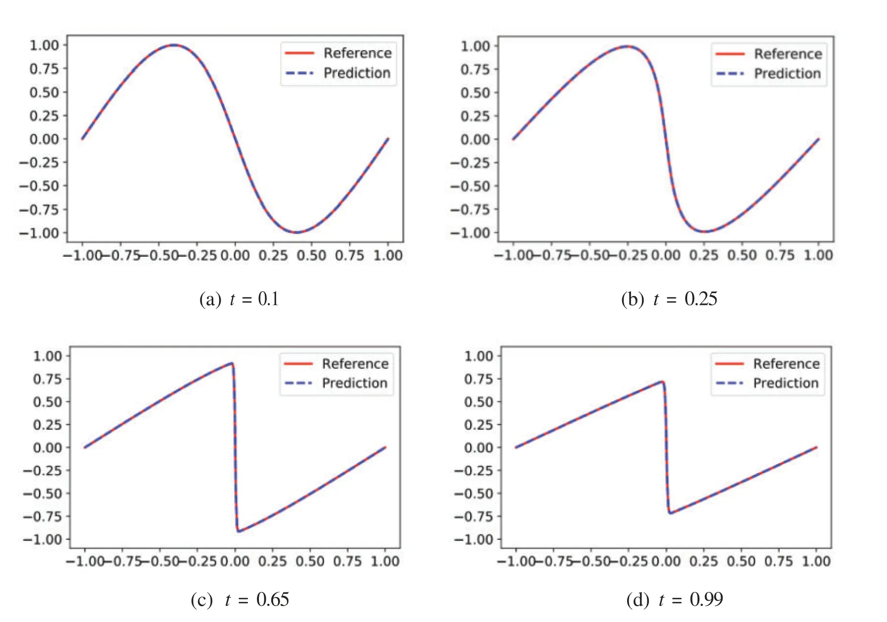
Figure 3:The comparison of predicted solutions obtained by LaNets and exact solutions at four time snapshots t=(0.1,0.25,0.65,0.99)for the one-dimensional Burgers equation

A more detailed numerical result is summarized in Table 1.It has to be noted that the early work[31]serves as a benchmark.In order to observe the influence of a different number of small sample points in the algorithm,we add 50 small sample points each time to calculate the corresponding results.From Table 1,one can visually see that the error of the LaNets model is one order of magnitude lower than that of PINNs.In addition, we can clearly find that 50 sample points used here can achieve a higher predictive accuracy than the 300 sample points used in the benchmark model.It means that using less label data to get more accurate predicted results is achievable, thereby saving a lot of manpower and material resources and increasing computational efficiency.

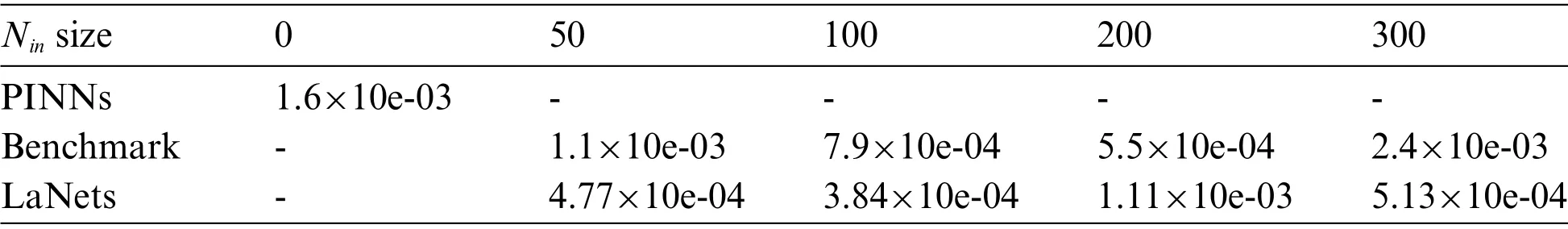
Table 1:The relative L2 errors for one-dimensional Burgers equation

3.1.2 Carburizing Diffusion Model

We consider the one-dimensional carburizing diffusion model[32]in Eqs.(9.1)–(9.4):

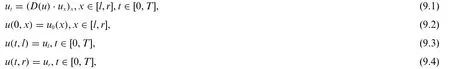
whereD(u)represents the diffusion coefficient anduis the concentration of carbon.Here,landrdenote the left and right boundary of the model.Diffusion is a fundamental process of carburizing,and the diffusion coefficient is related to temperature,the content of alloy elements,systems,etc.Next we consider carburizing diffusion equation with constant and variable diffusion coefficient,respectively.

1.Constant diffusion coefficient

We start with the constant diffusion coefficientD(u)according to Eq.(10):

whereD0,Q,RandT2are already given.In a practical sense,D0represents the pre-exponential factor,Qdenotes the activation energy of carbon,Rdescribes the gas constant andT2is the temperature during the carburizing process(K).

In this numerical experiment,we takeD0=16.2mm2/s,Q=137800J/mol,R=8.314J/(K×mol)andT2=1123K.The corresponding exact solution is written as Eq.(11):

where we haveup=1.2 andud=0.2.The terminal timeTof this model is 36000,the left boundarylis 0,and the right boundaryris 2.5.

Regarding the training set, we takeNu= 150,Nin= 300,Nf= 10000.Moreover, we employ a 8-layer LaNets to represent the solutionu(t,x)in this simulation.The LaNets model contains one Lagrange block, six hidden layers with 20 hidden neurons per layer and one output layer.Here, the relativeL2error is measured at 1.35×10-3.

In order to evaluate the performance of our algorithm in multiple ways,we compare the simulation results with the simulation results obtained by the PINNs model and our earlier model.The results for the three models are shown in Fig.4.We can clearly see that the predicted solution of the PINNs model is not quite consistent with the exact solution, and the differences become more and more obvious over time.And it is here that the LaNets model fits more accurately than the benchmark model.Thus,the proposed method has obvious advantages in the long time simulation of time-dependent partial differential equations.A more intuitive error value obtained by three algorithms is listed in Table 2,from which we find that the predicted error of the benchmark model is one order of magnitude lower than PINNs.Meanwhile,the predicted error of LaNets when using 300 sample points is almost one order of magnitude lower than the benchmark model.The decline curve of the loss function in the training process is shown in the Fig.5a.It can be seen that the loss has been declined to a small value in few iterations during the training process.

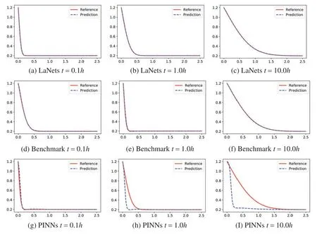
Figure 4:Predicted solutions for one-dimensional carburizing constant diffusion coefficient equation.Top row:LaNets model;Middle row:benchmark model;bottom row:PINNs model.First column:t=0.1 h;Middle column:t=1.0 h;last column:t=10.0 h

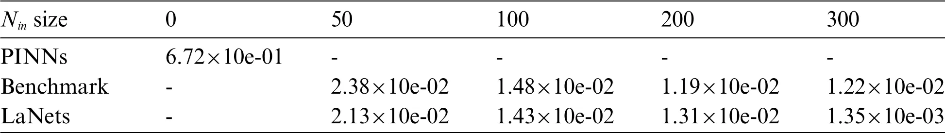
Table 2:The relative L2 errors for one-dimensional carburizing constant diffusion coefficient equation

2.Variable diffusion coefficient

In this experiment,the carburizing diffusion coefficientD(u)varies with the temperature,systems and ratio of the element.Here,we considerD(u)=cos u,and add a source terms(t,x)as Eq.(12):

The analytical solution corresponding to this setting is Eq.(13):

In this example,we haved= 0.5,the left boundaryl= -π,the right boundaryr=πand the ending timeT=1.Moreover,we use a 8-layer LaNets to denote the spatio-temporal solutionu(t,x).The curve of loss function during training is shown in the Fig.5b.

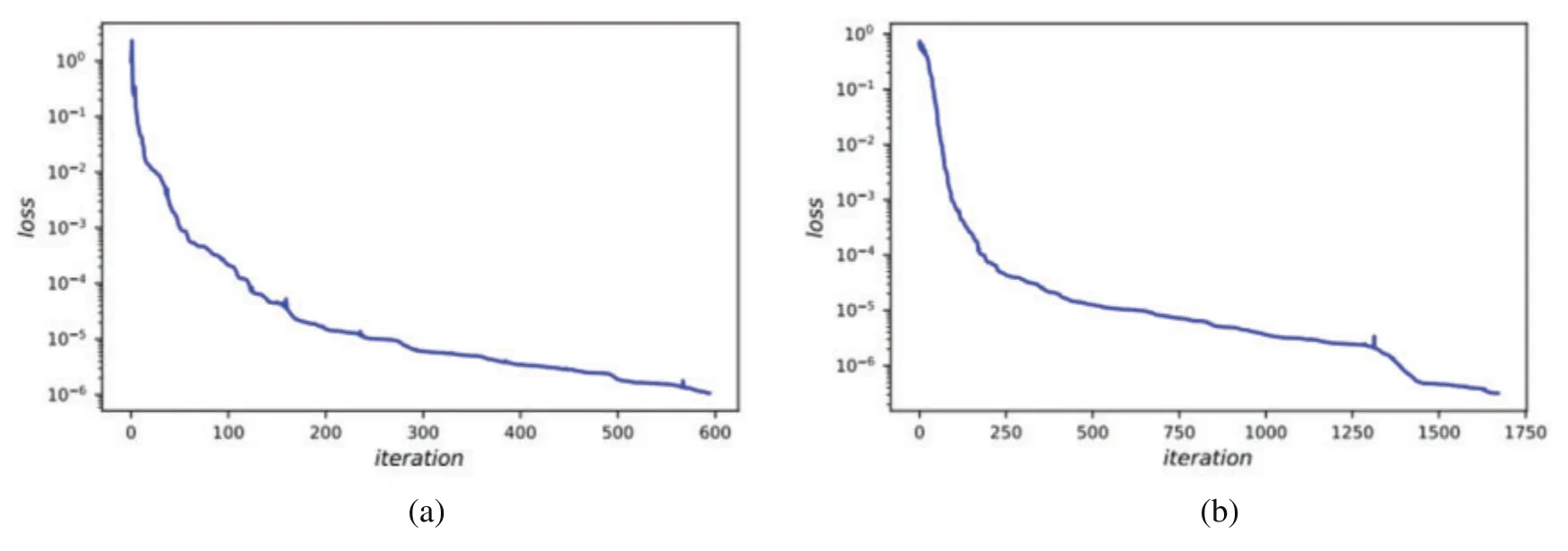
Figure 5:(a)The loss curve vs.iteration for the one-dimensional carburizing diffusion equation with constant diffusion coefficient.(b) The loss curve vs. iteration for the one-dimensional carburizing diffusion equation with variable diffusion coefficient

Further,we make a contrast between the simulation results obtained by the proposed model and the benchmark model.The detailed results for them are displayed in Fig.6.While all experimental results seem to be consistent with the analytical results,one can find that the predicted solution of the LaNets model is more closer to the exact solution.A more accurate error evaluation is summarized in Table 3,from which we see that the prediction error of the LaNets model is always lower than that of the benchmark model when using the same number of small sample points.

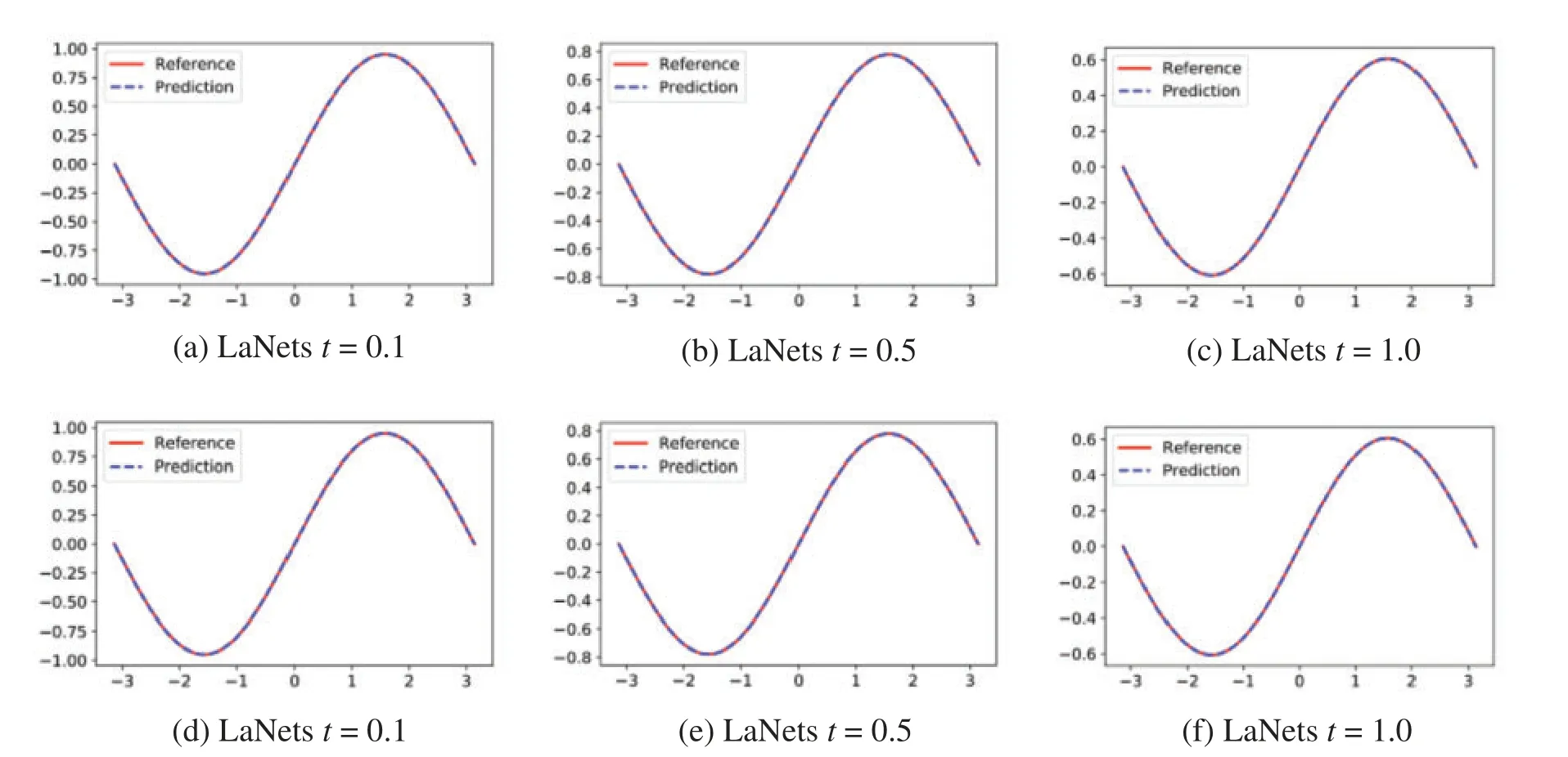
Figure 6:Predicted solutions for one-dimensional carburizing variable diffusion coefficient equation.Top row:LaNets model;bottom row:benchmark model.First column:t = 0.1;middle column:t =0.5;last column:t=1.0

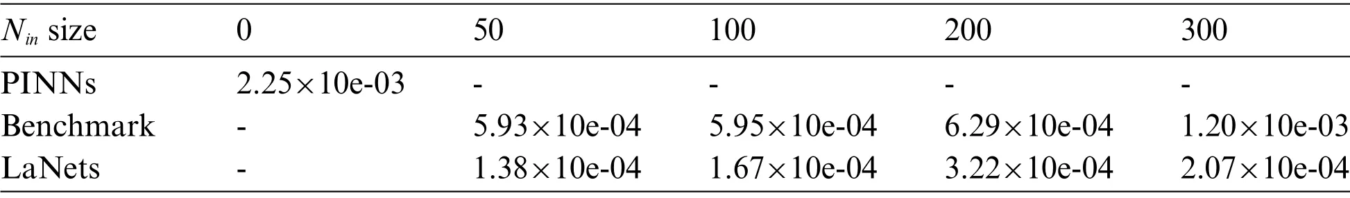
Table 3:The relative L2 errors for one-dimensional carburizing variable diffusion coefficient equation

3.2 Numerical Results for Two-Dimensional Equations

In this section,we consider two-dimensional problems including the time-independent Helmholtz equation and time-dependent Burgers equation to verify the effectiveness of the LaNets model.These two types of two-dimensional problems aim to demonstrate the generalization ability of our methods.

3.2.1 Helmholtz Equation

In this example,we consider a time-independent two-dimensional Helmholtz equation as Eq.(14):

with homogeneous Dirichlet boundary conditions and the source functionf(x,y)is given by Eq.(15):

Here,we takek=1 and the analytical solution is Eq.(16):

The training set of this example is generated according to the exact solution in the above equation.The problem is solved using the 4-layer LaNets model on the domain[-1,1]×[-1,1].And each hidden layer consists of 40 hidden neurons.The relativeL2error measured is 5.28×10-4.The training set is specified asNu=400,Nin=200,Nf=10000.

The visual comparison among LaNets,benchmark and PINNs results is displayed in Fig.7.From Fig.7,we find that the predicted solution of the benchmark model is not quite consistent with the exact solution.In addition,the proposed model is more accurate than the PINNs model especially on the boundary.Detailed error values for the three models are shown in Table 4,from which we see that the predicted error of the LaNets model is always minimal.The loss curve during the training process is shown in Fig.8a.From Fig.8a,we see that the value of the loss decreases continuously and smoothly from a higher value to a lower value,which shows the stability and robustness of the proposed model.

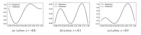
Figure 7:(Continued)

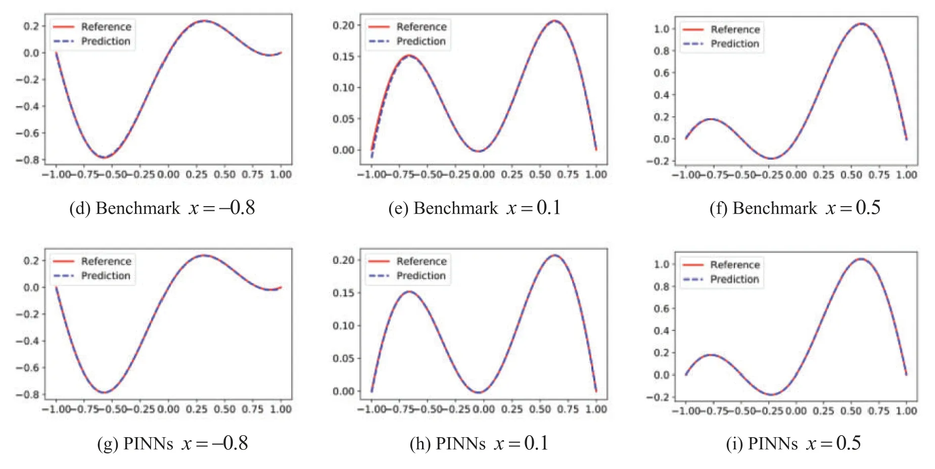
Figure 7:Predicted solutions for the two-dimensional Helmholtz equation.Top row:LaNets model;Middle row:benchmark model;bottom row:PINNs model.First column:x=-0.8;middle column:x=0.1;last column:x=0.5

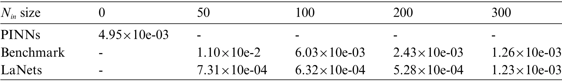
Table 4:The relative L2 errors for two-dimensional Helmholtz equation

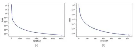
Figure 8:(a)The loss curve vs.iteration for two-dimensional Helmholtz equation.(b)The loss curve vs.iteration for two-dimensional Burgers equation

3.2.2 2D Burgers Equation

In the last experiment, we consider a two-dimensional time-dependent Burgers equation as Eq.(17):

whereurepresents the predicted spatio-temporal solution.The corresponding initial and boundary conditions are given by Eq.(18):

In this example,we takeλ= 0.1 andT= 3.The training set is generated by the exact solution Eq.(18),which is utilized to assess the accuracy of our method.The computing domain is set to[0, 1]×[0, 1] × [0, 3].We apply an 8-layer LaNets model and each hidden layer consists of 20 neurons.The residual training points are 20000 and the initial and boundary points are 150 whereas theNinpoints are 300.

The decline curve of the loss function is shown in Fig.8b.It can be seen that the loss value drops steadily to a small value over fewer iterations.Fig.9 displays the 3D plot of the solution att= 0.5,and the relativeL2error calculated is 2.06×10-4.The experiment of the two-dimensional timedependent Burgers equation proves that the proposed method can effectively solve high-dimensional time-dependent PDEs.In theory, the LaNets model can solve PDEs in arbitrary dimensions, and the remaining research is left for future work.The detailed relativeL2errors obtained by LaNets,benchmark and PINNs are given in Table 5, from which we can know that the predicted error of LaNets is lower than that of the benchmark model and PINNs model.

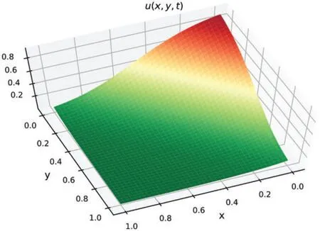
Figure 9:The predicted solution of the two-dimensional Burgers equation at t=0.5

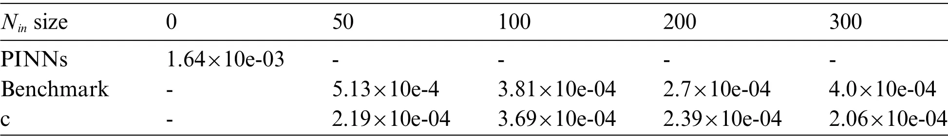
Table 5:The relative L2 errors for the two-dimensional Burgers equation

4 Conclusion

In this paper, we propose hybrid Lagrange neural networks called LaNets to solve partial differential equations.We first perform Lagrange interpolation through Lagrange block in front of deep feedforward neural network architecture to make pre-fitting and feature extraction.Then we add the residuals of small sample data points in the domain into the cost function to rectify the model.Compared with the single-layer polynomial network,LaNets greatly increase the reliability and stability.And compared with general deep feedforward neural network,the proposed model improves the predictive accuracy without adding any extra parameters.Moreover, the proposed model can obtain more accurate prediction with less label data,which makes it possible to save a lot of manpower and material resources and improve computational efficiency.A series of experiments demonstrate the effectiveness and robustness of the proposed method.In all cases,our model shows smaller predictive errors.The numerical results verify that the proposed method improves the predictive accuracy,robustness and generalization ability.

Acknowledgement:This research was supported by NSFC(No.11971296),and National Key Research and Development Program of China(No.2021YFA1003004).

Funding Statement:The authors received no specific funding for this study.

Conflicts of Interest:The authors declare that they have no conflicts of interest to report regarding the present study.