
Image Representations of Numerical Simulations for Training Neural Networks
2023-01-24 02:51YimingZhangZhiranGaoXueyaWangandQiLiu
Yiming Zhang,Zhiran Gao,Xueya Wang and Qi Liu
1School of Civil and Transportation Engineering,Hebei University of Technology,Tianjin,300401,China
2School of Computer and Software,Nanjing University of Information Science&Technology,Nanjing,210044,China
ABSTRACT A large amount of data can partly assure good fitting quality for the trained neural networks.When the quantity of experimental or on-site monitoring data is commonly insufficient and the quality is difficult to control in engineering practice,numerical simulations can provide a large amount of controlled high quality data.Once the neural networks are trained by such data,they can be used for predicting the properties/responses of the engineering objects instantly,saving the further computing efforts of simulation tools.Correspondingly,a strategy for efficiently transferring the input and output data used and obtained in numerical simulations to neural networks is desirable for engineers and programmers.In this work,we proposed a simple image representation strategy of numerical simulations,where the input and output data are all represented by images.The temporal and spatial information is kept and the data are greatly compressed.In addition,the results are readable for not only computers but also human resources.Some examples are given,indicating the effectiveness of the proposed strategy.
KEYWORDS Numerical simulations;neural network;pre-/post-processing;data compression
1 Introduction
With the recent developments of machine learning algorithms,frameworks and systems,numerous Artificial Neural Networks (ANNs) have been proposed,built and adopted rapidly and widely in engineering applications.Neural networks can be driven by mechanisms or data.The first type can be represented by the Physical-Informed Neural Network(PINN)[1,2],which uses control equations(commonly in the form of partial differential equations)for building objective and loss functions[3–5]and then finds the optimal solution in the approximation space[6].They are powerful tools for solving problems that are numerically unstable and time consuming for conventional methods such as finite element and mesh-free methods[7–9].The second type on the contrary are the neural networks driven by labeled data.The data can be obtained by on-site sensors,experiments and numerical simulations.In many cases,the knowledge behind the phenomena described by these data is unclear for the networks.On the one hand,the interpretability of such networks is unsatisfactory.On the other hand,these networks may help to reveal new patterns,rules,and knowledge by“learning”[10].Except for tools learning new patterns,data driven neural network can also be considered as a surrogate tool or a hierarchy model[11],as illustrated in Fig.1,taking the engineering design process as an example.In Fig.1,the blue arrows belong to the conventional design process and the red arrows belong to the design process augmented by data driven machine learning models.The green arrows belong to both.Once the machine learning models are trained,the large input-output database from parameter studies is unnecessary when the procedures in the frame can work independently and efficiently.
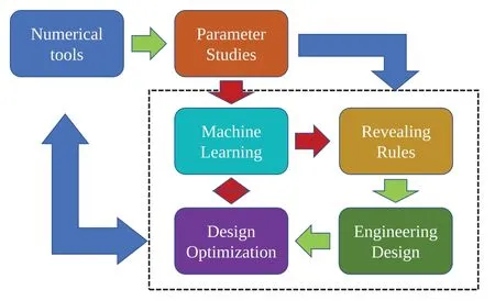
Figure 1:Date driven machine learning models in the engineering design process
Furthermore,engineering structures can be relatively large across space and time and the amount of data from on-site sensors and experiments,especially spatial data,is generally insufficient.In addition,these data can deviate considerably because of errors from monitoring or testing.In contrast,the quantity and quality of data from numerical simulations can be assured.Hence,first validating the numerical model by comparing the results to the experimental and monitored results and then training the neural network with numerically obtained data can be an advantageous procedure.
Basic data driven neural networks are sequential learning models.There are input and output datasets,between which the structures of the neurons can be assembled and built in the platforms associated with TensorFlow[12]and PyTorch.The lower bound of the number of datasets is problem dependent.Except for the design of neural networks,methods for efficiently transferring the datasets from numerical simulations to neural networks are necessary.In this work,considering the advantages of modern neural networks on graphic processing,we propose an image representation method of numerical simulations for training neural networks.The main features of the proposed method include:
· The method is easy to follow and can be implemented into the pre-and pro-processing parts of numerical tools such as those built in the finite element method(FEM)framework.
· The input images naturally take into account the spatial information of the cases,which can be understood by not only neural networks but also human resources.
· The sizes of the images can be further compressed/decompressed by other models such as autoencoders.
Some examples will be provided to show the flexibility and effectiveness of the method.Moreover,we want to emphasize here that some procedures we proposed in this work could be very basic and natural for researchers working in computational mechanics,who follow similar rules for pre-and proprocessing during programming and computing for a long time.Nevertheless,we believe the method can be inspiring and helpful for researchers and engineers working in other fields such as computer science,and civil and mechanical engineering,which is the main motivation of this work.In the next section,we will provide basic rules and examples together with which the procedures are clarified.
2 Method and Examples
2.1 Basics
We focus on 2D images and 2D simulations(planer or 1D transient cases)in this work,but the ideas can be extended to higher dimensional cases by using a series of continuous images/animations.Considering RGB images,every pixel has channels of three colors: red,green and blueRGB=[Rvalue,Gvalue,Bvalue].The value of each channel is between 0 and 255.A neural network was used for recognizing different compositions of heterogeneous materials represented by RGB images in [13],indicating that the information of RGB images including the RGB values as well as the pixel position can be properly transferred to neural networks.Herein,we take the numerical simulations conducted in the finite element framework as an example.The discretized domain is composed of elements,and each element has its own material and geometric properties.To ensure the performance of the neural network,only testable parameters can be considered as input parameters while the internal variables should not.
2.2 Mechanical Responses of Matrix-Inclusion Material
The mechanical responses of matrix-inclusion materials are basic numerical simulations for composites,such as concrete,rocks and polymers.The model and mesh are shown in Fig.2.The model will be loaded considering different boundary conditions including compression and shearing.As mentioned before,after large number of simulation results are obtained and transferred to neural network for training,the trained neural network can play the role of a database,which can provide mechanical responses of similar composites subjected to similar loading conditions.
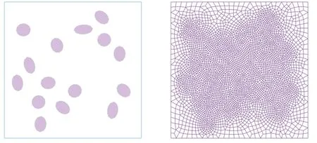
Figure 2:The model and mesh of the matrix-inclusion material
When the matrix and inclusion are isotropic and linear elastic,basic material properties include elastic modulus and Poisson’s ratio,represented by red and green channels as Eq.(1)
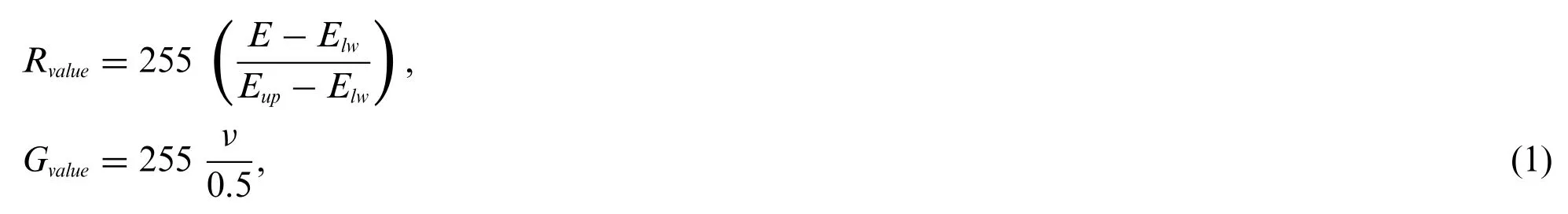
where(·)lwand(·)upare the lower and upper bounds of the corresponding parameters,respectively.The displacements along thexandydirections regarding isotropic and linear elastic conditions can be used for setting loading conditions,represented by red and green channels as Eq.(2)
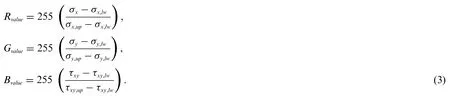
Meanwhile,the stress tensorσ=is the output parameter,occupying only three channels as Eq.(3)
It can be found that transforming the input/output parameters into RGB figures is a normalization step,which shall be done anyway for neural networks.
Considering the elastic modulus of the matrix and inclusion as 20 and 80 GPa respectively and the Poisson’s ratios of the matrix and inclusion as 0.3 and 0.1,respectively,the input and output images are shown in Fig.3,which includes compression and shearing conditions along thexandydirections.
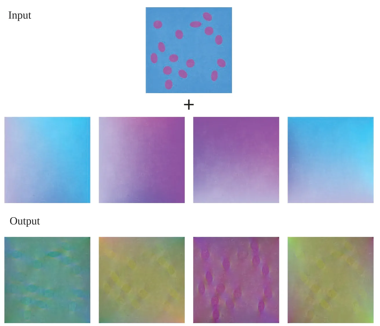
Figure 3:The input/output image representations of numerical simulations of mechanical responses of matrix-inclusion material with Elw = 10 GPa,Eup = 100 GPa,ux,lw = uy,lw = -0.05 mm,ux,up = uy,up =0.02 mm,σx,lw =σy,lw =-2.5 MPa,σx,up =σy,up =2 MPa,τxy,lw =-1 MPa,and τxy,up =1 MPa
2.3 Slope Stability
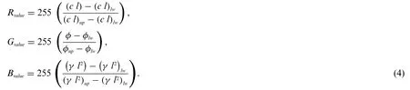
The second example refers to limit analysis of slope,which provides a factor of safety of a slope for assessing its stability and safety.Considering upper bound limit analysis,the necessary material parameters are cohesionc[kPa],friction angleφ[-] and weightγ[kPa/m].When slopes have very different sizes and these parameters are length scale dependent,normalizing the size of slopes before creating input images will be more convenient.We use the width of a slopelas the characteristic length and scale the slope into a width equal to 1.The material parameters become(c l)[kN],φ[-],and(γ l2)[kN],represented by three channels as Eq.(4)
The output results are represented by slip lines or so called failure pattern images,which are obtained by discontinuity layout optimization [14–19] in this example.Other methods such as the strength reduction method or other finite element limit analysis methods are also applicable[20–22].For illustration,the input and output images are shown in Fig.4.
Figure 4: The input/output image representations of numerical simulations of slope stability with1,500,000 kN
2.4 Coupled Thermo-Hydro-Chemical Analysis of Heated Concrete
When concrete members are subjected to fire loadings,explosive spalling may occur,which is the violent fracturing and splitting of concrete pieces from the heated structures.Spalling greatly jeopardizes the integrity and duratbility of structures[23],such as tunnel linings under fire accidents.Spalling is caused partly by the pore-pressure built up inside concrete,referring to the phase change,permeation and diffusion of liquid water and vapour [24–26] as a strongly coupled thermo-hydrochemical(THC)process.
The control equations of the THC model of heated concrete are composed of three strongly coupled heat equations,which need to be solved concurrently,as a computing exhausting numerical procedure.Meanwhile,the fire loadings and concrete properties can be complex.Engineers and designers would always like to quickly assess the spalling risk of specific structures considering different conditions,which is a strong motive for developing data driven neural network models.
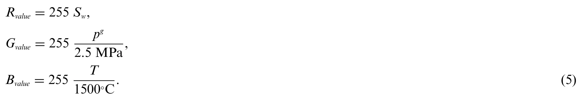
In[27],the authors summarized fifteen parameters referring concrete properties,fire loadings and environmental moisture as input parameters.In this work,we use grayscale images to represent these parameters.The output parameters are still represented by RGB images,where the saturation degreeSw,the pore pressurepg,and temperatureToccupy three channels as Eq.(5)
Considering the 1D case,the horizontal direction of the output image is taken for space distributions and the vertical direction is taken for time evolutions ofSw,pg,andT,see Fig.5.The input and output images are shown in Fig.6.
Figure 5:Using an RGB image for representing the time-space variations of Sw,pg,and T
Figure 6: (Continued)
Figure 6: The input/output image representations of numerical simulations of the coupled thermohydrochemical analysis of heated concrete
3 Numerical Example for Training a Neural Network by Images
3.1 The Structure of the Neural Network
A hybrid neural network composed of an autoencoder(AE)and a fully connected neural network(FNN) was built by the authors for learning the coupled THC example in [27].In this work,we simplify the structure and use a network composed of a convolutional neural network (CNN) and a fully connected neural network (FNN).Three designs are considered,see Figs.7 to 9,which are used for learning the data provided in Subsection 2.4 as examples.CNN can process images efficiently which is composed of convolution and pooling layers,where the convolution layers can extract features and the pooling layers can compress the data.Design 1 has four convolution layers and no pooling layer.Design 2 has three convolution layers and two pooling layers.Design 3 has four convolution layers and three pooling layers.In our example,the CNN is expected to extract and compress features from the input images containing concrete material parameters,environmental humidity and fire load.The FNN is used to build the mapping relation from the features to the output images containing the pore pressure,temperature and saturation information.For both CNN and FNN,the layer plays the role of building the mapping relation from the input vector X to the output vector Y as Eq.(6)

where W and b are the weights and biases respectively used in this layer.f(·)is the activation function.For the FNN,the input vector and output vector are fully connected.In other words,each element of X influences each element of Y.In contrast,CNN uses a filter in the mapping process that slides at a defined step and outputs the sum of the product[28].
Taking the structure shown in Fig.9 as an example,the CNN-FNN hybrid neural network is similar to an autoencoder(AE).The CNN plays the role of an encoder when the FNN plays the role of a decoder.There are 6720 sets of input and output images in the example,90%of which were used as training sets and 10%as test sets.The number of convolution kernels of the first three convolution layers is 16,32,64,and the size of the convolution kernels is 3 × 3.A pooling layer is added after each of the first three convolution layers.The size of the feature map after pooling is 128,64,32.The fourth convolution layer contains a convolution kernel with size 1×1,further reducing the dimension of the feature vector.The compression rate of the CNN is 0.13%.The FNN has three hidden layers to amplify the feature vector to the output images,which is similar to the work we presented in[27].The optimizer of the network is the Adam optimizer,and the stochastic gradient descent method is used.The MSE with regularization term is chosen as the loss function as Eq.(7)

λis the regularization hyper-parameter andλ=10-4used in this work.Piis the real image vector and Siis the predicted image vector.qis the number of output images.
Figure 7:The structure of neural network 1
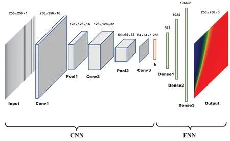
Figure 8:The structure of neural network 2
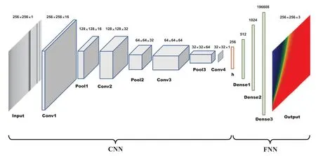
Figure 9:The structure of neural network 3
To avoid over-fitting,the K-fold cross-validation method is used to verify the generalization capability of the model.The 6048 groups of input and output images of the training set were divided into 10 groups of disjoint subsets and trained 10 times.Each time,one group was selected as the verification set and the other 9 groups were selected as the training set.Ten groups of data were trained and evaluated.The average loss and standard deviation obtained from ten-fold cross validation were 0.002295(±0.000171).Table 1 summarizes the hyperparameters used in the network.It is worth mentioning that numerous designs can be considered.We are still working on improving the designs,which will be presented later.
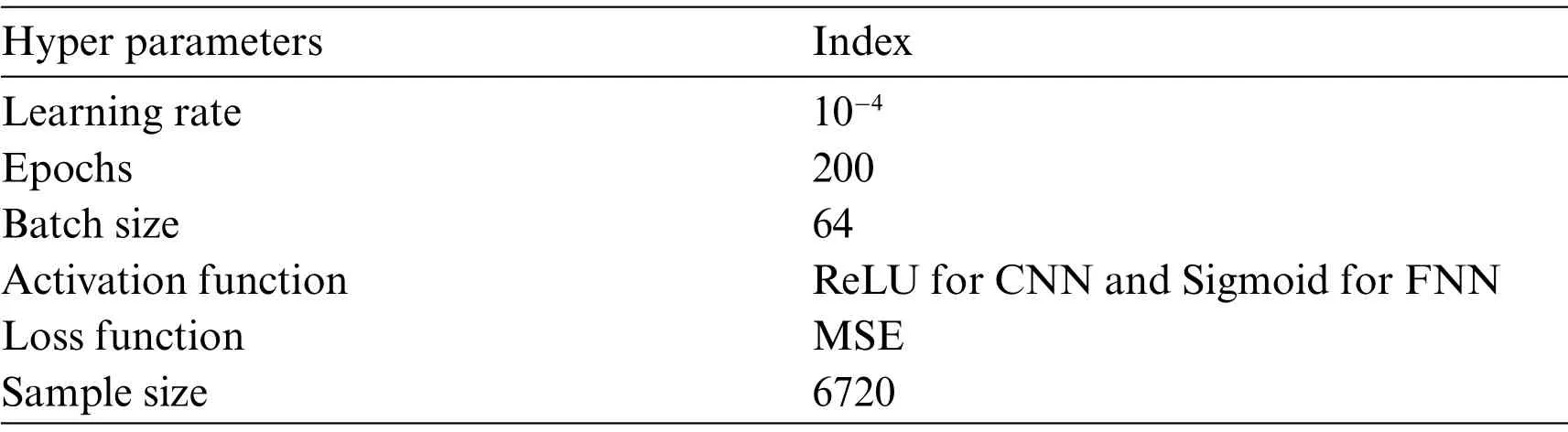
Table 1: List of hyperparameter of the hybrid autoencoder neural network
3.2 Results
The evolution of the MSE loss with the evolution time(epoch)of all designs considering training and testing are shown in Fig.10.For all designs,the MSE loss drops very fast in training as well as testing.The original,and predicted results and their errors are shown in Figs.11 to 13,where the original images do not belong to the training or testing data.The error images are generated with corresponding pixel values of 255-|P-S|.The results indicate that the shapes are captured and that the colors are very similar.However,some details do not agree very well,especially in regions with high gas pressure.The errors can be further reduced by increasing the amount of data.Generally,design 3 provides the best results.We would like to emphasize that although the results are generally satisfying for the coupled THC example,the design of the network is mostly case dependent.When learning new data sets,the procedure to design,compare,test,and improve the network shall be conducted once more.Some recently proposed networks indicate that it is possible to build some widely applicable networks[29],which uses a similar design for a large number of scenarios.The researchers only need to adjust the hyperparameters.Some research is still ongoing.Except for the design of the network,increasing the number of data sets can effectively improve the prediction accuracy,which can be time consuming.
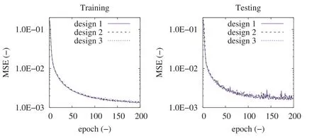
Figure 10:The learning and testing results considering different network designs
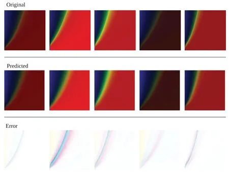
Figure 11:The original,predicted and error images of design 1
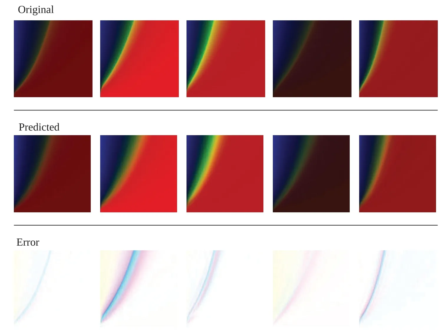
Figure 12:The original,predicted and error images of design 2
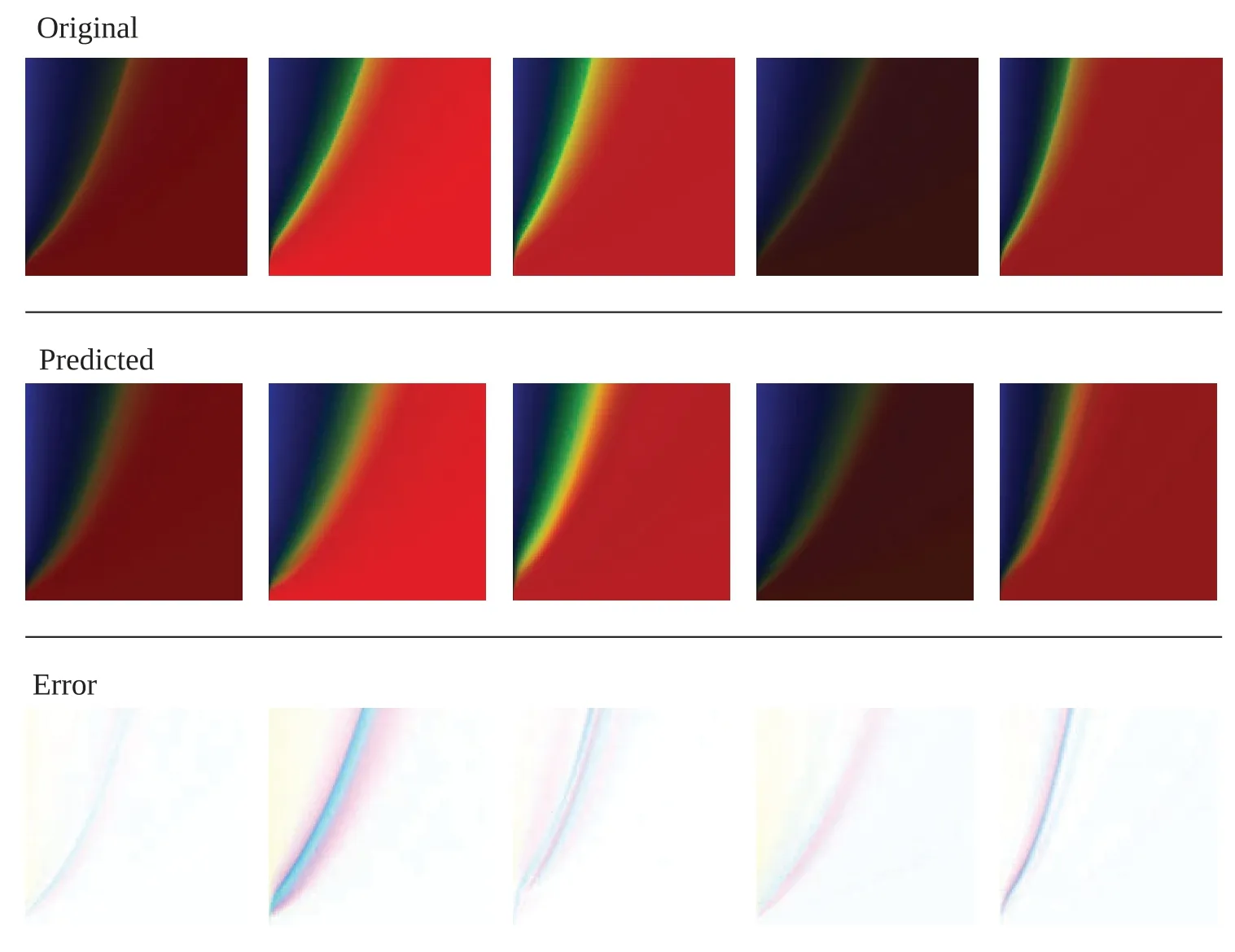
Figure 13:The original,predicted and error images of design 3
4 Conclusions
In this work,we present a strategy for representing the input parameters and output results of numerical simulations by images.With several examples we show that this strategy is simple and compatible with the pre/post-processing parts of popular numerical tools.The images account for the spatial and temporal information used and obtained in the numerical simulations.In addition,all images can be reprocessed by other algorithms.For one of the examples,we train a hybrid CNN-FNN neural network with the input/output images,indicating the effectiveness of the proposed strategy.
Funding Statement:The authors gratefully acknowledge the financial support from the National Natural Science Foundation of China(NSFC)(52178324).
Conflicts of Interest:The authors declare that they have no conflicts of interest to report regarding the present study.
 Computer Modeling In Engineering&Sciences2023年2期
- Computer Modeling In Engineering&Sciences的其它文章
- Detecting Icing on the Blades of a Wind Turbine Using a Deep Neural Network
- Optimizing Big Data Retrieval and Job Scheduling Using Deep Learning Approaches
- Structural Damage Identification Using Ensemble Deep Convolutional Neural Network Models
- Self-Triggered Consensus Filtering over Asynchronous Communication Sensor Networks
- State Estimation Moving Window Gradient Iterative Algorithm for Bilinear Systems Using the Continuous Mixed p-norm Technique
- Refined Sparse Representation Based Similar Category Image Retrieval