Topology Optimization of Sound-Absorbing Materials for Two-Dimensional Acoustic Problems Using Isogeometric Boundary Element Method

Jintao Liu,Juan Zhao,★and Xiaowei Shen,2,★

1College of Architecture and Civil Engineering,Xinyang Normal University,Xinyang,464000,China

2College of Mechanics and Materials,Hohai University,Nanjing,211100,China

ABSTRACT In this work,an acoustic topology optimization method for structural surface design covered by porous materials is proposed.The analysis of acoustic problems is performed using the isogeometric boundary element method.Taking the element density of porous materials as the design variable,the volume of porous materials as the constraint,and the minimum sound pressure or maximum scattered sound power as the design goal,the topology optimization is carried out by solid isotropic material with penalization (SIMP) method.To get a limpid 0–1 distribution,a smoothing Heaviside-like function is proposed.To obtain the gradient value of the objective function,a sensitivity analysis method based on the adjoint variable method (AVM) is proposed.To find the optimal solution,the optimization problems are solved by the method of moving asymptotes(MMA)based on gradient information.Numerical examples verify the effectiveness of the proposed topology optimization method in the optimization process of two-dimensional acoustic problems.Furthermore,the optimal distribution of sound-absorbing materials is highly frequency-dependent and usually needs to be performed within a frequency band.

KEYWORDS Boundary element method;isogeometric analysis;two-dimensional acoustic analysis;sound-absorbing materials;topology optimization;adjoint variable method

1 Introduction

With the rapid development of road and railway construction and the rapid increase in car ownership,noise pollution is increasingly affecting our lives and health,which has become a worldwide problem.Researchers have introduced several methods for optimizing design,including a range of work on sound barriers [1–3],automobiles [4–6],buildings [7,8] and mufflers [9,10].At present,porous materials have been widely used in the field of noise control because of their excellent sound absorption characteristics[11–15].Considering various constraints,including economy,laying porous materials in certain areas is an effective method.Therefore,it is necessary to obtain the partial optimal distribution of porous materials under given constraints.This leads to a series of problems about topology optimization[16–18].Since Bendsøe et al.[19]proposed the topology optimization method,which has become an important engineering tool.Many researchers have also introduced topology optimization techniques into acoustic analysis[20–23].Topology optimization of the distribution of porous materials in two-dimensional muffler models using the finite element method (FEM) was first proposed by Yoon et al.[24],and the framework was extended to the topology optimization of acoustic barrier surfaces composed of both rigid and porous materials by Kim et al.[1].However,it is a typical semi-infinite domain external sound field problem,and it is difficult to numerically simulate the performance of the noise barrier by the FEM.As we all know,the boundary element method(BEM) is superior to the FEM when solving sound field problems in infinite/semi-infinite domains because of its advantages such as high accuracy and automatic mesh generation[25–28].However,as the amount of computation increases,the process of meshing will consume a lot of costs,which makes the transition process from CAD to CAE very cumbersome.When encountering dynamic computation processes,the mesh needs to be constantly reconstructed.In isogeometric analysis(IGA)[29,30],the spline basis function commonly used in CAD is used to replace the Lagrangian basis function in the traditional interpolation form,which successfully eliminates the transformation process from CAD to CAE[31,32].At the same time,geometric errors are eliminated and therefore the accuracy of the calculation is significantly improved.The BEM can be well combined with IGA due to the discrete nature of BEM,that is,the isogeometric boundary element method(IGABEM)[33–35].IGABEM not only retains the advantages of the BEM such as dimensionality reduction and high accuracy but also enables numerical analysis to be carried out directly from CAD,which greatly improves calculation efficiency [36–39].Therefore,IGABEM is chosen for the optimal analysis of acoustic problems in this work.

As we all know,the solution methods of optimization problems are mainly the non-gradient method and the gradient method.The non-gradient method has no use for gradient information,i.e.,the derivatives of the objective and constraint function in regard to the design variables.Moreover,the non-gradient algorithm can achieve better solutions for problems with fewer degrees of freedom such as dimensional optimization,while the solution efficiency is very low for problems with a large number of degrees of freedom such as topology optimization.However,the gradient algorithm is well-efficient for large-scale problems,thereby,most extension optimization problems are solved by the gradient algorithm.From an engineering point of view,the gradient method is obviously more practical because it can save the cost.In addition,the gradient algorithm requires gradient information(i.e.,sensitivity information)of the objective function and constraints in regard to the design variables to guide the iterative update of the design variables during optimization.Therefore,it is necessary to solve the gradient value of the objective function.The finite difference method (FDM) [40–42] performs a differential operation on each design variable to get complete gradient information.Therefore,its computational efficiency is highly dependent on the number of design variables.In addition,the accuracy of FDM depends largely on the step length and the computational accuracy of the objective function itself.Too large or too small a step length will affect the results of the calculation,and the stability is difficult to be guaranteed in the actual calculation.Compared with FDM,the direct differentiation method(DDM)[43–45]uses chain differentiation rules to get the gradient value for the objective function on the basis of intermediate gradient values.The DDM is easy to understand and highly stable,so this method is widely used for sensitivity analysis.However,as the number of design variables increases,DDM requires a computer with high storage capacity.In summary,neither FDM nor DDM applies to problems with a large number of degrees of freedom.Compare with DDM,the adjoint variable method(AVM)[46,47]can avoid the calculation of gradient values for intermediate variables by introducing adjoint equations.And the adjoint equations are independent of the design variables.Therefore,AVM tends to be less costly and more suitable for solving optimization problems with a large number of design variables.Numerous scholars have introduced the AVM into structuralacoustic sensitivity analysis,and have achieved remarkable results[48–50].

Among the various methods of topology optimization of continuums,the variable density method is the most widely used.Because this method makes the original 0-1 discrete design problem into a continuous design problem,and then it is easier to solve it using mathematical methods.Currently,the solid isotropic material with penalization (SIMP) and the rational approximation of material properties (RAMP) are common interpolation methods in the variable density method.In addition,topology optimization methods based on them have been widely used [51–53].Bendsøe et al.[54]utilized the SIMP method to achieve geometric parameterization and implemented topology optimization of single and multi-material structural designs.Bendsøe[55]utilized the SIMP method to eliminate the discreteness of elasticity problems for shape optimization.Li et al.[56] utilized the RAMP method to eliminate numerical instability in the process of topology optimization and solve the problem of the structural heat transfer design.Because the SIMP method has the advantages of high computational efficiency and simple concept,this work proposes an optimization method that combines the boundary element method and the SIMP method to optimize the distribution of sound-absorbing materials.Design variables are then updated using the MMA method to find the final optimal solution[2,57].

The rest of the work is arranged as follows.NURBS is briefly introduced into Section 2.Section 3 is the basic formulations for BEM.Section 4 describes the whole optimization process,including the creation of the topology optimization model,material interpolation method,the analysis of the acoustic sensitivity and updating schemes for design variables.Section 5 provides several numerical examples to verify the availability of the proposed optimization procedure.Section 6 elaborates the conclusions of this work.

2 B-splines and NURBS

Using the concept of the knot vector,the B-spline basis functionNi,sis defined as follows:

where the knot vector is denoted asΞ= [ξ0,ξ1,···,ξm],ξi∈R is thei-th knot,mis the number of nodes of the knot vector,m=n+s+1,sis the polynomial order,andnis the number of basis functions or control points.Eqs.(1)and(2)are often referred to as the recursive formula.

Non-Uniform Rational B-Splines (NURBS) [2,31] developed from B-splines,is an important geometric modeling technique in CAD and is considered as an industry standard.Therefore,all geometries in this work are represented by NURBS.The NURBS curve x(ξ)takes the form as Eqs.(3)–(5)

where NURBS basis functionsRi,s(ξ)are defined as

with

wherewiis the weight associated with the control point Si.

3 BEM for 2D Acoustic Analysis

The Helmholtz governing differential equation based on sound pressure is shown as Eq.(6)

wherep(x)is the sound pressure,kis the wave number.To eliminate non-unique solutions at a series of virtual eigenfrequency points,the linear combination [58] of the conventional boundary integral equation (CBIE) and the hyper-singular boundary integral equation (HBIE) takes the form shown below:

whereαis defined asi/kfork≥1,andiotherwise.q(y)=∂p(y)/∂n(y)is the unit outward normal vector at pointy,and the coefficientC(x)=1/2 if the source pointxlies on a smooth boundaryS.pincis the sound pressure of the incident wave.The expression of the kernel functions presented in Eq.(7)are as Eq.(8)

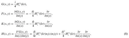
wherer=|x-y|,is then-th order Hankel function of the first kind.

For 2D half space problems,the kernel functions can be expressed as Eq.(9)

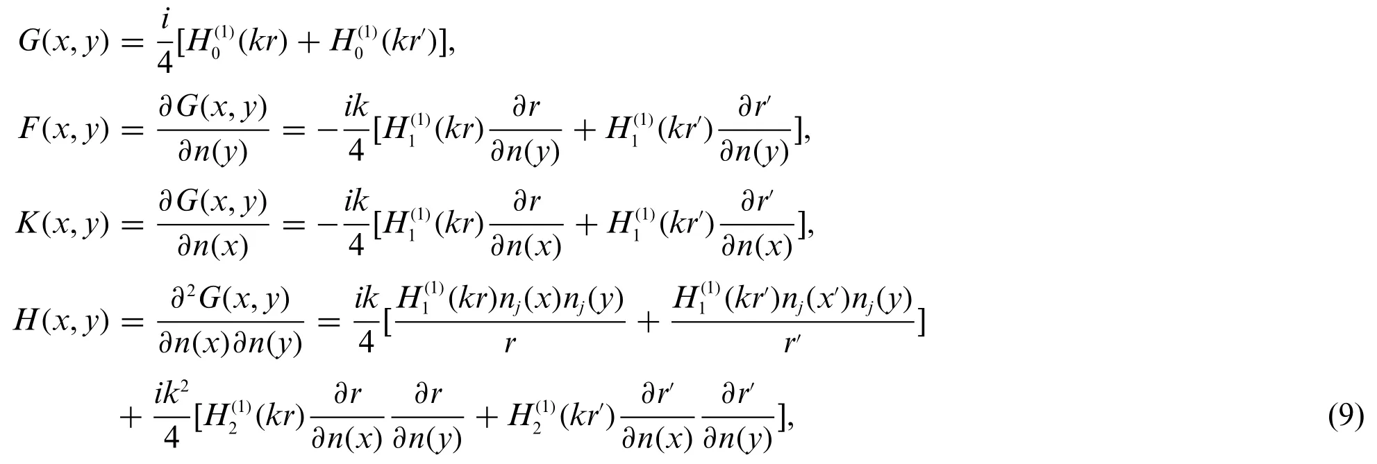
in whichr′is the distance fromx′toy,x′is the symmetric node of source pointx.H(x,y)andG(x,y)have strong singularity and weak singularity,respectively,where the first term in the integral forH(x,y)can be solved using the singular elimination technique based on the Guiggiani method andG(x,y)can be solved using logarithmic Gaussian integration.WhileF(x,y)andK(x,y)have no singularities,this work is solved using Gaussian integration.

In this work,we utilize NURBS to discretize the boudary of the structure.The Eq.(7) are discretized into matrix form as Eq.(10)

where coefficient matrices H and G of the system equation are full rank,asymmetrical.After introducing the boundary condition,the Eq.(10)can be simplified to

where A is the coefficient matrix,z is the unknown vector,and b is the known vector.By solving Eq.(11),we can obtain the unknown vector z.Therefore,using Eq.(7)withC(x)= 1,we obtain the sound pressure vector at several points lying on the acoustic domainΩ,as Eq.(12)

where coefficient matrices Hfand Gfbelong to the acoustic domainΩ.

4 Topology Optimization Model Based on BEM

4.1 The Creation of Topology Optimization Model

The topology optimization problem that obeys the material volume constraint can generally be expressed as Eq.(13)

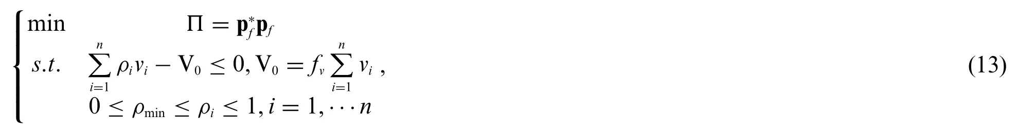
whereΠis the objective function with respect to the sound pressure,pfis the sound pressure vector for the field points,is the conjugate transpose of pf.ρiandviare the volumetric density and volume of element i (i= 1,···n),respectively,ρminis the lower bound of the volume density to avoid the occurrence of singular values during calculation,V0is the volume constraint.

Taking into account the impedance boundary conditionq(x)=ikβ(x)p(x),the Eq.(12)can be expressed as Eq.(14)

in which B is a diagonal matrix,which can be expressed as Eq.(15)

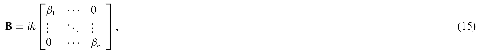
whereβiis the normalized admittance of thei-th element.

4.2 Material Interpolation Scheme

To solve the problems that the design variables between 0 and 1 are discrete,the relationship between the normalized surface admittance valueβ0and the material densityf(ρi)ati-th element is described to Eq.(16)

in which the admittance of thei-th element is marked asβi.And the SIMP interpolation function[54]is introduced as Eq.(17)

in whichγ=3 is the penalization factor,which can make the intermediate density close to 0 or 1.

4.3 The Analysis of Acoustic Sensitivity

In the previous section,the admittance has become a continuous function,therefore the optimization problem can be solved using gradient-based algorithm.In this work,AVM is used for the analysis of acoustic sensitivity.Firstly,the derivative of the objective function regarding the design variable is divided into three parts as Eq.(18)

where ℜ represents the real part of the complex number,andz3are instrumental variables.After the discrete forms of the boundary integral equation and the integral equation in the domain are substituted into the objective function,the new objective function can be denoted as

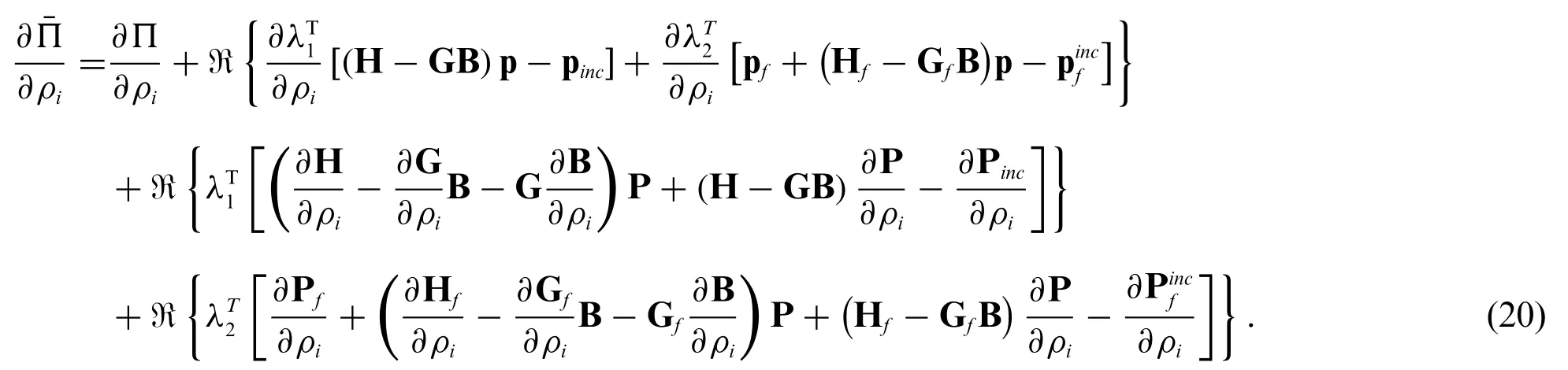
Actually G,H,Gfand Hfhave nothing to do with the design variables,thereby the derivative terms of these coefficient matrices can be vanished directly.In addition,we also assume that the external excitation remains unchanged during the optimization process,and then there are∂pinc/∂ρi= 0 and=0.Hence,the Eq.(20)can be simplified as

Substituting the Eq.(21) into the Eq.(18) and letting the adjoint vector satisfy the following adjoint equation:

After solving the Eq.(22) to obtain the adjoint vectors,the derivative of the objective function regarding any design variable can be expressed as Eq.(23)

In acoustic optimization,a number of different objective functions can be chosen,including sound pressure value,radiated power and transmission loss.In this work,two different objective functions are used for the optimization analysis.

Objective function 1:To obtain the minimum sound pressure,the objective function is shown as Eq.(24)

Objective function 2:To obtain the maximum the absorbed sound power of the sound-absorbing materials,the objective function is shown as Eq.(25)

whereW0=1×10-12is the reference the sound power,andWis the sound power absorbed by soundabsorbing materials.

4.4 Design Variable Updating Method

In this work,the topology optimization problem is solved using MMA [57].The flowchart of topology optimization process based on acoustic IGABEM is shown in Fig.1,the convergence condition is as Eq.(26)

whereΠjis the objective function value of thej-th iteration step,τrepresents the relative error of convergence.

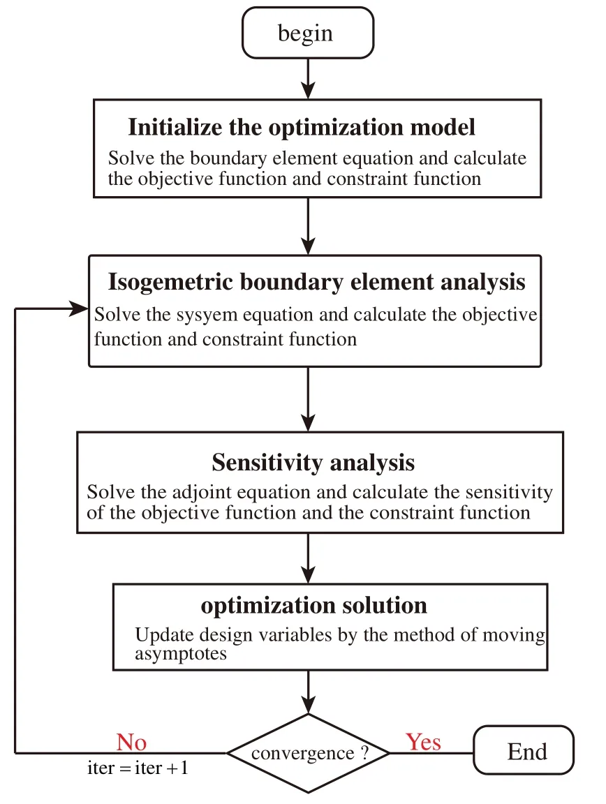
Figure 1:The flowchart of topology optimization process based on acoustic IGABEM

5 Numerical Example

To investigate the effectiveness and applicability of the proposed optimization method,this section presents some numerical examples.In all examples,the boundary integral equations are discretized with the constant element.In addition,this work implements the topology optimization algorithm using Fortran 95 code.To improve computational efficiency,the OpenMP technique is employed to parallelization.The following analysis of the acoustic problems is performed on a desktop computer with an Intel Core i5-10400 CPU and 8 GB RAM.In this work,the number of Gaussian quadrature points utilized for regular integrals is 6 and 10 Gaussian quadrature points are used for singular integrals.

5.1 Half-Y Shaped Sound Barrier

In this work,we consider a computational domain of the half-Y shaped sound barrier as shown in Fig.2.The width of the sound barrier is 0.2 m,the height of the upright part is 2.8 m,the height of the inclined part is 2 m,and the inclination angle is 60°.The point excitation is located at(0 m,1 m)and the distance from the sound barrier is 10.4 m.The ground is simplified to a rigid surface,so the problem can be simplified to a two-dimensional half-space problem,at which the basic solution is shown in Eq.(9).The excitation frequencyfpis set to 70 Hz.Relevant parameters are shown in Table 1.In the following numerical study,we set the minimum value of design variablesρminand the iterative convergence conditionτto 0.001 and 1.0×10-4,respectively.

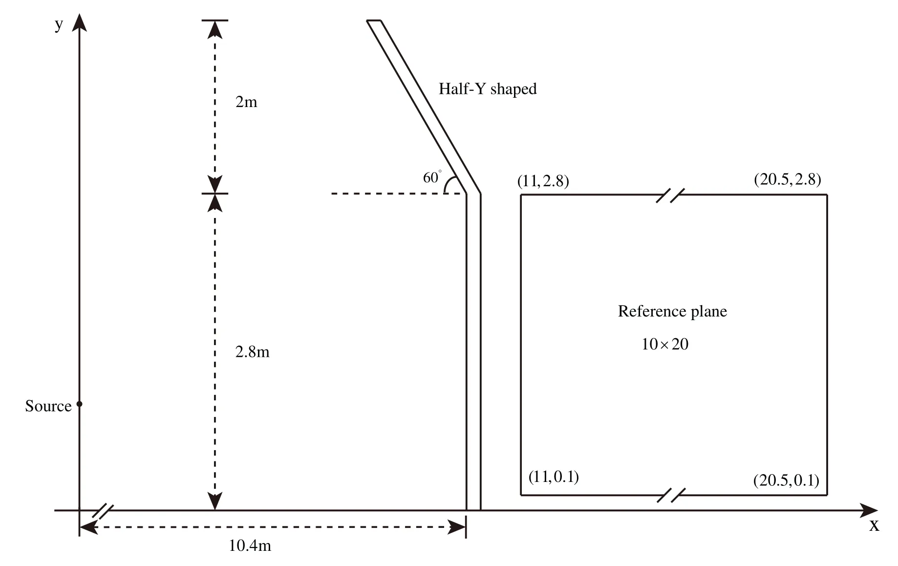
Figure 2:The computational domain of the half-Y shaped sound barrier and reference plane

Table 1: Relevant parameters for the sound barrier design example

Firstly,the topology optimization analysis is performed with MMA to verify its effectiveness.The initial values of design variables are set to 0.5,the volume ratio of sound-absorbing materials is bound to 1 and the penalization factorγis set to 3.Fig.3 shows the trend of objective function values and volume fraction of the sound-absorbing material over the iteration step during optimization iteration.It can be seen that the final value of the optimized objective function is significantly lower than the initial value,and the final convergent material volume fraction is much lower than the given constraint value(full coverage of sound-absorbing material).Furthermore,Fig.3 demonstrates a steady decrease of the objective function and the volume function in the iterative process.This phenomenon shows that the more sound-absorbing materials,the lower the objective function is,and the optimized local distribution of sound-absorbing materials has a better noise reduction effect than the full coverage distribution of sound barrier surface for the objective function 1 defined in this example.The volume constraint ratio obtained by using MMA is about 0.617.Therefore,the full coverage of soundabsorbing materials fails to achieve the best noise reduction effect,which illustrates the necessity for the optimal distribution of sound-absorbing materials on the surface of the sound barrier.

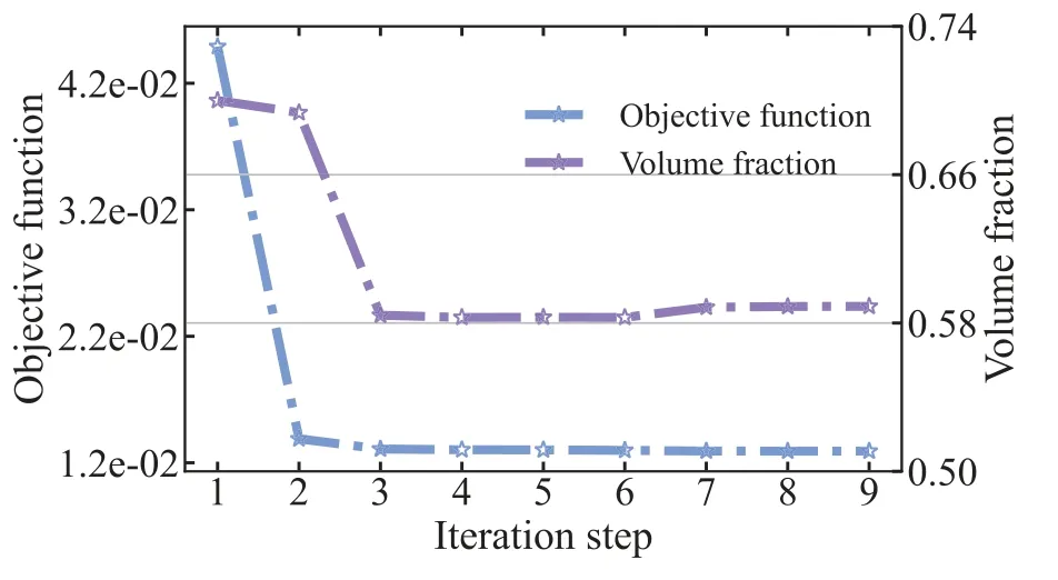
Figure 3:Objective function and volume fraction of half-Y shaped sound barrier at 70 Hz

It can be seen from Fig.3 that the volume constraint changes very smoothly at the optimal solution.To examine in detail the reasons for the appearance of this phenomenon,the values of the sensitivity of all elements are given in Fig.4 for the initial value,iteration step=3 and iteration step=6.From Fig.4,we can see that the values of the sensitivitiy can be either positive or negative.When the values of the sensitivity are positive,increasing the number of design variables will increase the values of the objective function.Otherwise,the values of the objective function will be reduced.Fig.5 shows the distribution of design variables and values of the sensitivity after optimization convergence.It can be seen that the sensitivity values of many elements are zero after convergence,but there are still some parts that are non-zero.The reason is that the range of variation between the upper and lower bounds of the design variables makes it impossible for the sensitivity values to converge to zero,which is also the difference between unconstrained and constrained optimization.

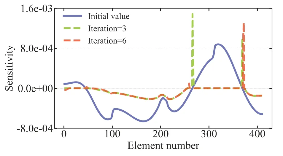
Figure 4:Distribution of the sensitivity value in the optimization process

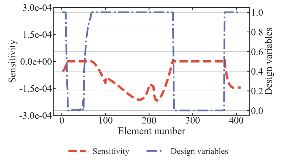
Figure 5:Distribution of design variables and sensitivity values after optimization convergence

Fig.6 shows the optimal distribution of sound-absorbing materials on the surface of the sound barrier for different iteration steps during the optimization process,including the optimization iteration step=0,the optimization iteration step=4,the optimization iteration step=8,and final optimization convergence.The dark part indicates that the element is covered with sound-absorbing materials,and the design variable is 1.The light-colored part indicates that the element is rigid,and the design variable is 0.When the design variable is between 0 and 1,it means that the element is in an intermediate density state,namely the gray element.Grey element usually has no practical physical significance and is only the intermediate value introduced when using the variable density method,which should be avoided in topology optimization.To get a limpid 0-1 distribution,a smoothed Heaviside-like function based on the SIMP method is used to punish the intermediate density.As can be seen from the figure,there are almost no gray elements after convergence.Therefore,the proposed objective function 1 can produce a clear layout.

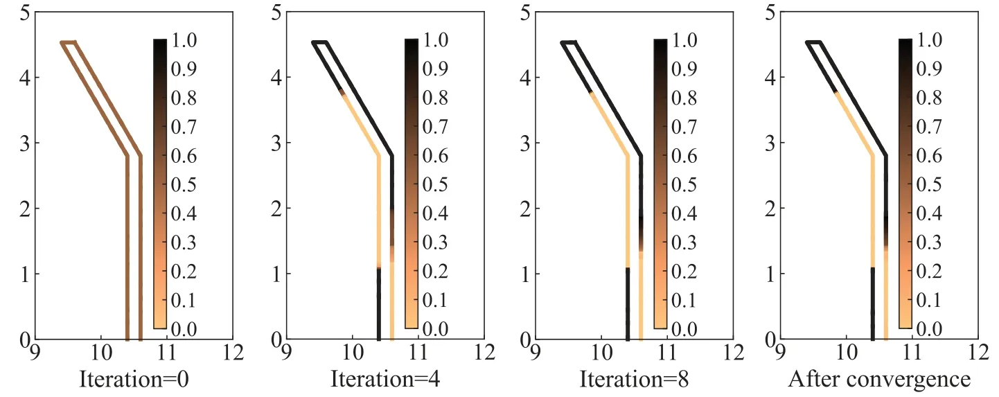
Figure 6: Distribution of sound-absorbing materials on the surface of half-Y shaped sound barrier under different iteration steps

As the optimization algorithm that we use iteratively updates the design variables with the help of the first-order gradient values of the objective function 1,we can only find locally optimal solutions,but there is no guarantee that the solution is a globally optimal solution.To ensure the global optimization of the solution,several different initial values are usually selected to obtain different optimization results,and the one with the best performance is selected as the final solution.Although this method can not guarantee that the final result is the global optimal solution,it can avoid some poor local optimal values to a great extent,and at least guarantee that the final result is better.Fig.7 shows the trend of the objective function and volume fraction with different initial values at 70 Hz.In the figure,nine different initial values are selected,namely design variablesρi=0.1,0.2,0.3,0.4,0.5,0.6,0.7,0.8 and 0.9.Fig.8 shows the optimized distribution of the corresponding sound-absorbing materials.

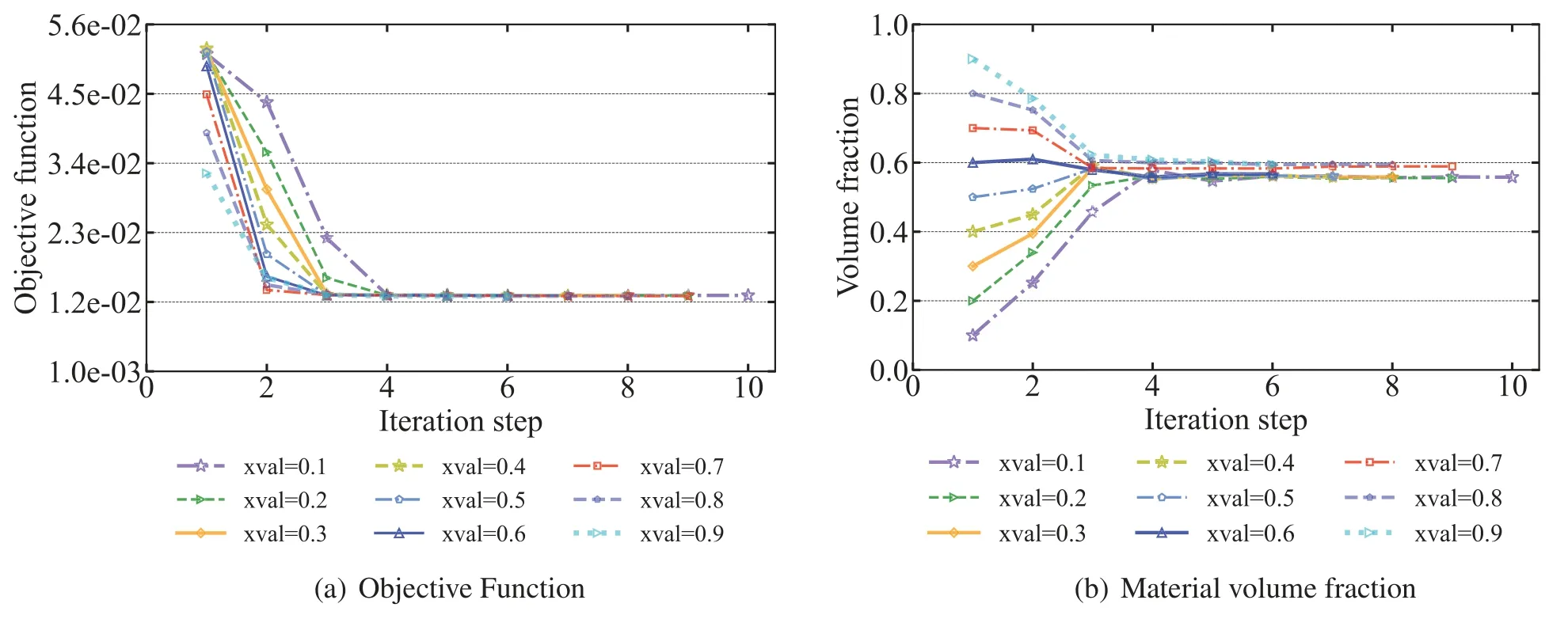
Figure 7: Objective functions and material volume fractions of sound barrier volumes for different initial values at 70 Hz

As can be seen from Fig.7b that the volume fraction of the final optimized distribution obtained by using a relatively high initial value is correspondingly higher.As can be seen from Fig.8 when the initial values are chosen between 0.7 and 0.9,the final optimized distribution is very similar and the corresponding volume fractions in Fig.7b are very close to 0.6.However,when the initial values were taken from 0.1 to 0.6,the optimized distribution was missing a piece in the lower right of the sound barrier compared to other optimized distributions.The volume fraction is between 0.5 and 0.6,and the corresponding objective function values are a little higher than other objective function values.It means that if the initial value is too small,it is possible to converge to the extreme value where the volume fraction is too small,and the original purpose of optimization cannot be achieved.In general,it is recommended to choose a relatively large initial design variable.In addition,we find that the optimized distribution obtained when the initial value is 0.9 is the highest volume fraction.However,there is no advantage over the optimized distribution of the initial values of 0.7 and 0.8.Therefore,different initial values lead to different optimization results.

To investigate the effect of frequency on the optimized distribution,we calculate the optimized distribution of sound-absorbing materials on the surface of the sound barrier at 70,140 and 210 Hz,as shown in Fig.9.As can be observed in the figure,the optimized distribution of sound-absorbing materials obtained at three different frequencies is different.This suggests that the optimized distribution is frequency-dependent and varies as frequency increases.As the frequency rises,the wavelength becomes shorter and the phase change period on the surface of the sound barrier becomes shorter.The interference of scattered and incident waves will be more dramatic between the two states of phase length and phase extinction interference,thereby the aggregated blocks of sound-absorbing materials on the surface of the sound barrier will become shorter and periodically distributed.

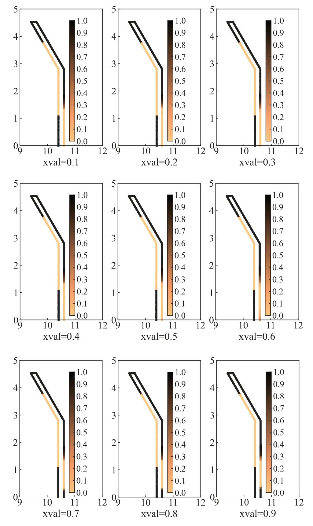
Figure 8:Optimized distribution of sound-absorbing materials for different initial design variables

Figure 9:Optimized distribution of sound-absorbing materials for different frequencies

Since the optimized distribution is frequency-dependent,an optimized distribution at one frequency point may simply be better or even worse at other frequencies.And the actual noise usually contains components of different frequencies and intensities.Therefore,it is of engineering significance to consider the objective function in a frequency band range.The new objective function can be defined as Eq.(27)

whereflandfuare the lower and upper limit of the frequency band,respectively.Πnewis the value of the objective function at multiple frequency points.The sensitivity values of the objective function regarding the design variables can be solved in the same way as the sensitivity values of a single frequency point.

The optimized distributions of sound-absorbing materials are given in Fig.10 for three different frequency bands,including 70-210 Hz,210-410 Hz and 410-610 Hz,which will be referred to as “layouts 1”,“layouts 2” and “layouts 3” in the subsequent analysis.It can be found that these three optimized distributions are significantly different from those obtained at 70,140 and 210 Hz,and the optimized distributions are also very different at different frequency bands.This means that the optimized distribution in the sense of frequency band also depends on the selected frequency band range.The optimized distribution at the frequency band has more overall significance within the examined frequency band compared to the optimized distribution at a single frequency point.Furthermore,due to the high-frequency range of the calculations,e.g.,“layouts 3”,the optimized distribution of sound-absorbing materials on the left side of the barrier is very fragmented.Finally,it should be noted that the optimized distribution of sound-absorbing materials in the respective frequency bands has been given in Fig.10.But this does not mean that each of these frequency points distributed within the frequency band performs best,and they perform the best only in the average sense of the entire frequency band.

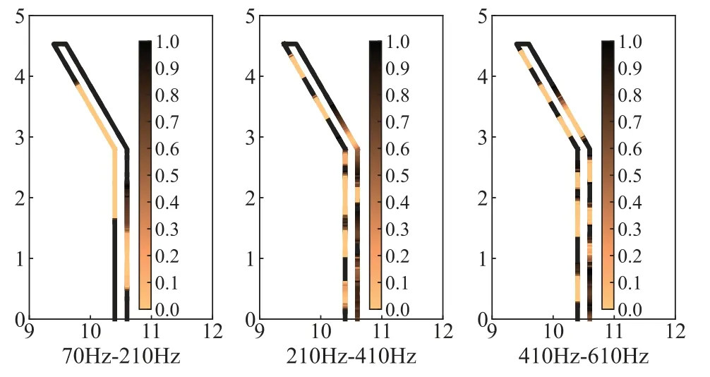
Figure 10:Optimized distribution of sound-absorbing materials in different frequency bands

5.2 One Circle

In this section,to further detect the feasibility and effectiveness of the proposed topology optimization algorithm for different acoustic problems,a numerical analysis of a computational domain consisting of a plane incident wave and an infinite cylinder is carried out.This can be simplified to a two-dimensional problem,as shown in Fig.11.The circle is discretized using 4,000 elements,thereby,the total degrees of freedom(DOF)is 4,000.Relevant physical parameters as shown in Table 2 and the volume constraintfvis 0.5.The iterative convergence conditionτis set to 10-5and the excitation frequency is 400 Hz.

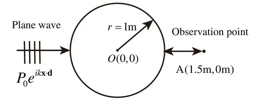
Figure 11:Computational domain of the optimization problem

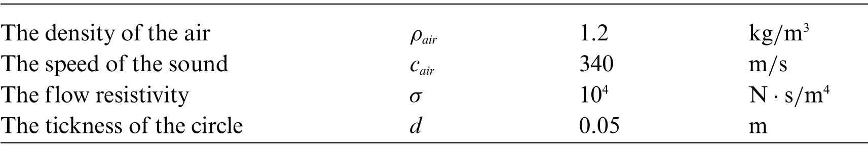
Table 2: Related parameters for the circle design example

Subsequently,we consider the optimization problem under the action of a plane waveP0eikx·d.The plane wave propagates along thexaxis,the incident direction vector is d =(1,0),and the amplitudeP0is set to 1,as shown in Fig.11.To minimize the sound pressure at point A and maximize the absorbed sound power of sound-absorbing materials,it is necessary to topologically optimize the distribution of the porous material.While more design variables lead to better solutions,they are also more likely to lead to the checkerboard phenomenon that lacks practical engineering significance in optimal solutions.Therefore,the circle is discretized using 4,000 elements in this work.At the same time,the volume fraction constraint is set to 0.5 and the initial value of design variables is set to 1.Fig.12 shows the trend of two different objective functions and the corresponding volume fractions of porous materials during the optimization process.Since the set volume fraction constraint is much smaller than the given initial value,the volume fractions corresponding to the two objective functions drop sharply in the second iteration step.And objective function 1 converges to a volume constraint value equal to near 0.4 and objective function 2 converges to a volume constraint value equal to near 0.5.The objective function 1 has a significant increase in the second step,while the objective function 2 decreases sharply at the beginning of the optimization.The two different objective functions show a steady decline and an increasing tendency,respectively,finally converging to the optimized value.In addition,we observe that the optimized objective function 1 is lower than the initial objective function 1,while the optimized objective function 2 is similarly lower than the initial objective function 2.This indicates that the optimized distribution of porous material performs better in terms of local distribution compared to the initial value of full coverage.This phenomenon can also be observed in the previous section for the optimized distribution of sound-absorbing materials on the surface of the sound barrier.The main reason is that the physical quantities of the sound field are complex variables,and the interference between the complex variables makes the contribution of the design variables to the objective function bidirectional.The previous section confirmed this by observing the presence of positive and negative values for sensitivity values during the optimization process.When applying a material-covered design,the objective function values for the inactive elements are higher than the objective function values for the non-inactive elements.In this work,we demonstrate the existence of inactive elements.Therefore,the distribution of porous materials needs to be optimized.

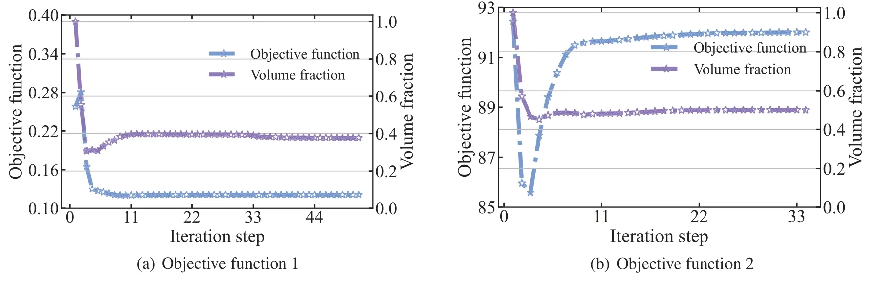
Figure 12:Objective function and volume fraction of the circle at 400 Hz

The optimized distributions of sound-absorbing materials after convergence are represented in Fig.13.The optimization results for objective function 1 are shown in Figs.13a and 13b shows the optimization results for objective function 2.The shade of color in the figure represents the relative magnitude of the design variable,where dark color indicates that the design variable is 1 and light color indicates that the design variable is 0.From the figure,it can be found that the optimized distribution obtained by the two different objective functions is completely different.The purpose of the optimal distribution of sound-absorbing materials is to find the optimal impedance boundary conditions so that the incident and scattering waves achieve the optimal interference in the sense of optimizing the target.When different objective functions are chosen,the corresponding optimal interference is often different.Therefore,the final optimized results are usually different as well.It can be observed from Fig.13b that the vast majority of sound-absorbing materials are distributed in the left half-circle.This is mainly because the plane wave is located on the left side of the circle,so the sound pressure value on the left half-circle is higher than that on the right half circle.At this time,the sound-absorbing materials are organized in the left half-circle to absorb energy more efficiently.In addition,as the optimized area,the excitation and the examination point A are all symmetric about thexaxis,the optimization results are also symmetric about thexaxis.There are almost no intermediate density elements in both optimized distributions,which indicates that the adopted filtering function can effectively eliminate the intermediate density.

Figure 13:Material topology optimization distribution of the circle at 400 Hz

The sound field distribution on the boundary and in the region of an infinite cylinder is shown in Figs.14 and 15,respectively.The selection of the observation point is consistent with the location of the observation point in Fig.11,and the remaining parameters are the same as those in Table 2.We consider several different frequencies of the incident plane wave,includingf= 100,150,200,250,300,350,400,450,500,600,650,700,800 and 900 Hz.It can be seen from the figure that the distribution of the sound pressure of porous materials is highly frequency-dependent,and its spatial distribution becomes more complex with the increase of incident frequency.In addition,the range of maximum and minimum sound pressure is not consistent for different objective functions.The sound field distribution on the boundary and in the region of an infinite cylinder is symmetric concerning thexaxis.Subsequently,we similarly considered the topologically optimized distribution of sound-absorbing materials for different frequencies,as shown in Fig.16.It can be seen from the figure that the distribution is different for different frequency points,which is consistent with the previously observed frequency-dependent.Although there are differences in the optimized distribution obtained at different frequency points,the basic distribution is very similar.Most porous materials are distributed in the left half-circle,as shown in Fig.16b.Fig.16 shows that the optimized distribution of the porous material is symmetric about thexaxis.

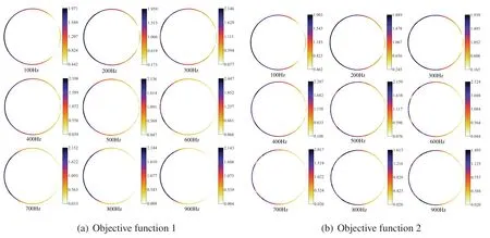
Figure 14:Distribution of the sound pressure for different frequencies

In this work,the influence of the location of the observation point on the optimization result is investigated,and only objective function 1 is affected by the observation point.First,we consider six different observation points,as shown in Fig.17.The computational frequency and other parameters are kept the same as before.Fig.18 shows the optimized distribution of porous materials obtained by six different observation points when objective function 1 is selected.The optimized distribution of the six different observation points is significantly different,which indicates that the optimized distribution of sound-absorbing materials is very sensitive to the location of the selected observation point.The sound pressure at the observation point is determined by the interference between the incident and scattered waves,which in turn is influenced by the phase of the incident and scattered waves.Therefore,when the position of the observation point changes,the sound propagation path changes accordingly,which further results in a phase change.The final porous material needs to be adjusted according to the phase,etc.,thus the optimized distribution depends on the chosen observation point.In addition,it can be observed that five observation points deviate from thexaxis,so the corresponding optimized distribution is no longer symmetric about thexaxis.

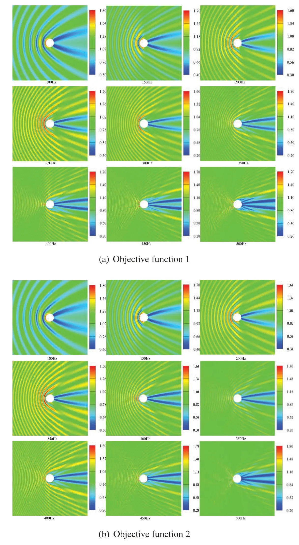
Figure 15: Optimized distribution of the sound pressure in the external sound field at different frequencies

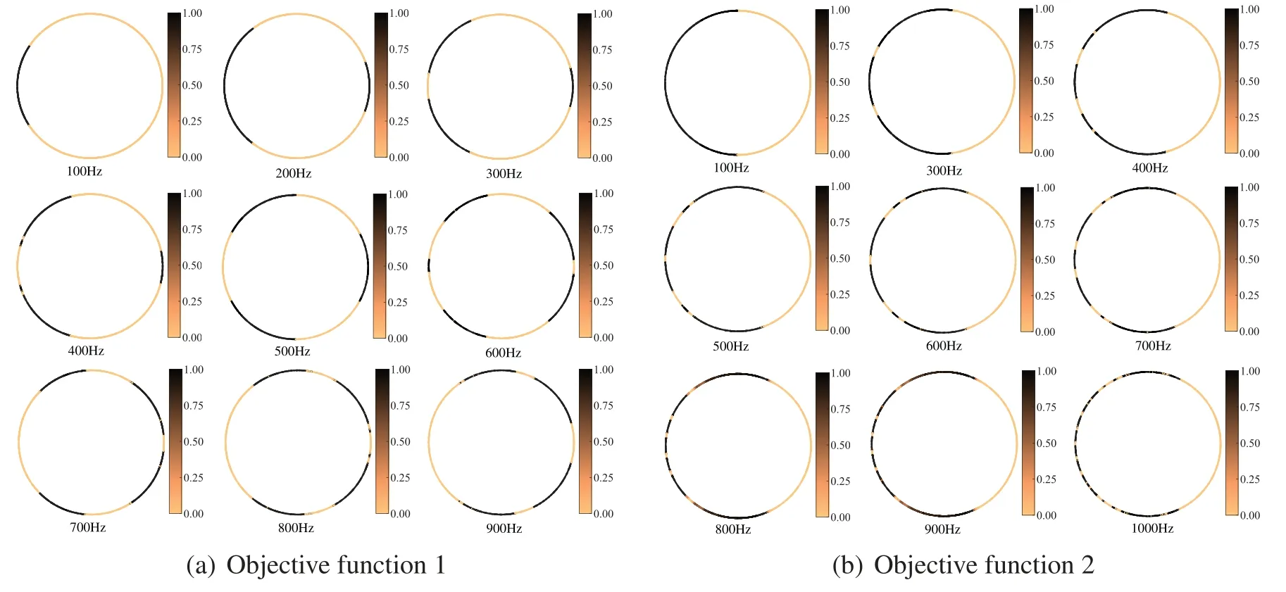
Figure 16:Material topology optimization distribution of the circle for different frequencies

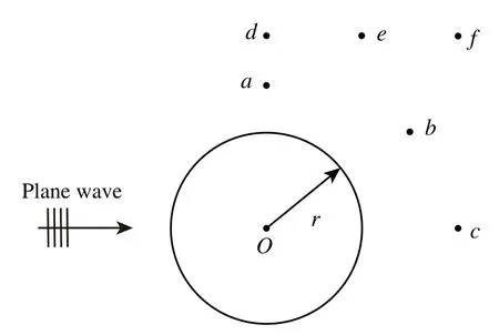
Figure 17:A model of the circle for different observation points

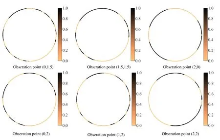
Figure 18:Optimized distribution of porous materials for different observation points

6 Conclusions

This work establishes a topology optimization method for porous sound-absorbing materials based on the acoustic IGABEM.The effectiveness of the algorithm is verified by numerical examples and the influence of frequency and location of the observation point on the optimization results is discussed.By analyzing results of different studies,we can draw some conclusions as follows:

1.The optimal distribution of the sound-absorbing material usually depends on the objective function chosen,so the optimized distribution is usually different for different objective functions.

2.Since the optimization distribution is frequency-dependent and location-dependent of the observation point,the optimization under the frequency band and the selection of multiple points or certain areas for investigation become more necessary and more engineering.

Acknowledgement:Thanks the editors of this journal and the anonymous reviewer.

Funding Statement:This work is sponsored by Natural Science Foundation of Henan under Grant No.222300420498.

Conflicts of Interest:The authors declare that they have no conflicts of interest to report regarding the present study.