A Hybrid BPNN-GARF-SVR Prediction Model Based on EEMD for Ship Motion

Hao Han and Wei Wang

School of Instrumentation and Optoelectronic Engineering,Beihang University,Beijing,100191,China

ABSTRACT Accurate prediction of ship motion is very important for ensuring marine safety,weapon control,and aircraftcarrier landing,etc.Ship motion is a complex time-varying nonlinear process which is affected by many factors.Time series analysis method and many machine learning methods such as neural networks,support vector machines regression (SVR) have been widely used in ship motion predictions.However,these single models have certain limitations,so this paper adopts a multi-model prediction method.First,ensemble empirical mode decomposition(EEMD)is used to remove noise in ship motion data.Then the random forest(RF)prediction model optimized by genetic algorithm(GA),back propagation neural network(BPNN)prediction model and SVR prediction model are respectively established,and the final prediction results are obtained by results of three models.And the weights coefficients are determined by the correlation coefficients,reducing the risk of prediction and improving the reliability.The experimental results show that the proposed combined model EEMD-GARF-BPNN-SVR is superior to the single predictive model and more reliable.The mean absolute percentage error (MAPE) of the proposed model is 0.84%,but the results of the single models are greater than 1%.

KEYWORDS Back propagation neural network; ensemble empirical mode decomposition; genetic algorithm; random forest;SVR;ship motion prediction

1 Introduction

Under the influence of wind,waves and other factors,the movement of the ship sailing on the sea in six degrees of freedom is randomly complicated and it seriously affects the sport safety of the ship.Since it is difficult to establish an accurate dynamical model for ship motion,most of the existing models for predicting ship motion are based on the measurements data of the ship at historical moments to predict the movement in the future.

There are a lot of studies that have been adopted in ship motion prediction.These methods are mainly categorized into traditional time series analysis methods and intelligent prediction methods.Traditional methods mainly include auto-regressive model (AR),moving-average model (MA) and auto regressive moving average mode (ARMA).Yumori et al.established ship motion prediction model based on AR and ARMA model with measured information,including wave motion and ship motions[1].And similar models can be found in Zhang et al.[2,3].However,these methods generally used the least squares to solve model coefficients but it was inappropriate to use this constant model coefficients to forecast ship motion which is a random process.Therefore,Peng et al.proposed a method for on-line estimation of parameters using recursive least squares and developed an on-line fast ARMA fixed-order algorithm[4].The methods mentioned above play an important role in predicting the ship motions,but AR,MA and ARMA model are linear models,which are not suitable to forecast the real ship motion which has complex,strong nonlinear and chaos characteristic.

Huang et al.creatively proposed a new processing method called empirical mode decomposition(EMD),which can effectively and adaptively deal with the nonlinearity and non-stationarity existing in actual engineering signals[5].EMD is to equalize the original time series with the sum of several stationary intrinsic mode function (IMF) components and a trend function component,which is the process of smoothing the original time series.Therefore,it has been popularly employed in developing hybrid models for various time series prediction.Huang et al.proposed AR-EMD technique decomposing the complex ship motion data into a couple of simple intrinsic mode functions and residual,which produces better prediction compared to AR models [6].Duan et al.developed a hybrid AR-EMD-SVR model which overcomes the non-stationary difficulty and achieves better predictions than other models[7].However,the EMD method has mode mixing and endpoint effects,which destroys the physical meaning of the IMF.Aiming at the deficiency of EMD,EEMD is adopted in this paper to decompose complex signals of ship motion into multiple simple sub-signals[8,9].

With the development of artificial intelligence technology,machine learning models,which could solve the nonlinear or nonstationary problem,have drawn attention and are used to predict the time series.These models are all data-driven models,such as Artificial Neural Networks(ANNS),Support Vector Regression(SVR),etc.Zhang et al.discussed diagonal recurrent neural network and acquired better results[10].Peng et al.proposed a novel method of single-output three-layer Back Propagation(BP)neural network to identify Volterra series kernels,which has higher precision,longer prediction time,effectiveness and adaptability [11].Huang et al.applied radial basis function (RBF) neural network to develop one-step forward prediction of ship pitching motion [12].Peng et al.proposed Echo State Network(ESN)based on Kalman filter algorithm for modeling in ship motion.However,there are issues that must be considered regarding the actual number of hidden nodes included in an ANN [13].Liu et al.introduced a prediction method based on extreme learning machine,support vector machine and particle swarm optimization (PSO-KELM),which has a simple structure,fast training speed and simulation results showed high accuracy prediction[14].Luo et al.adopted support vector machine for the parametric identification of ship coupled heave and pitch motions with real oceanic conditions[15].Furthermore,Li et al.designed a dynamic seasonal robust v-support vector regression forecasting model(DSRvSVR)and analysis results showed that the hybrid model received better forecasting performance compared with other models [16].Ensemble learning tree model is another important machine learning model that has achieved great success in predicting weather,stocks,traffic flow[17,18].For example,Chen designed a random-forest based forecast model that had consistently shown better predictive skills than the ARIMA model for both long and short drought forecasting [19].Li et al.adopted the ARIMA-XGBooost hybrid model to forecast China’s energy supply security level and got accurate result[20].But tree model is rarely used to predict ship motion.

Due to the uncertainty of ship motion,the methods mentioned above usually use a single complex model for prediction,which becomes unreliable when overfitting or failure occurs.Therefore,an EEMD-GARF-BPNN-SVR combined prediction method is proposed in the paper,which can effectively utilize the information of different single models and has higher precision and credibility.The final prediction result is obtained by adding the results of various models according to the weight coefficient.And the weights coefficients are determined by the correlation coefficients.

The rest of this paper is structured as follows:First,the EEMD algorithm and various prediction models are introduced.The methods used to predict ship motion are introduced in detail,including time series method and various machine learning algorithms such as BPNN,SVR,RF and XGBoost.Then the GA algorithm for optimizing RF model parameters and the combined prediction model based on correlation coefficient are introduced.Next,all the models are constructed with measured data and the performance of each model is analyzed.The conclusion is drawn finally.

2 Method

In general,the goal of the prediction model is to map historical data(xt,xt-1,···,xt-p)to future dataxt+qwith mapping functionf:

wherepis the number of the inputs,qis the prediction step size.Due to the non-stationary and nonlinear behavior of ship motion,fis a time-varying nonlinear function.Therefore,ship motion prediction is a nonlinear multi-step prediction problem which is more difficult than one-step ahead forecasting,since it has to deal with various additional complications,like reduced accuracy and increased uncertainty[21,22].

In this paper,the EEMD-BPNN-GARF-SVR algorithm is used as the prediction model.Fig.1 shows the main framework of the algorithm proposed in this paper.

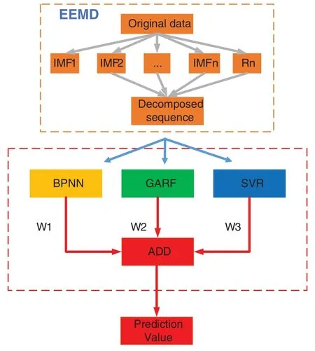
Figure 1:The framework of the EEMD-BPNN-GARF-SVR model

First,original data is processed by EEMD and is divided inton+1subsets includingIMFi(i=1,2,...n)and a residual set.IMF1corresponds to the highest frequency component andIMFncorresponds to the lowest frequency component.IMF1is considered as a noise sequence,thus a reconstructed sequence can be obtained by removingIMF1.Then the reconstructed data is divided into training set and test set.training set is used to build BPNN,GARF and SVR models,where the parameters of GARF is optimized by genetic algorithm (GA),and the test data is used to test the prediction performance of the models.The final prediction results of the hybrid model are obtained by combining the results of single model,while the optimal weighting coefficients are determined according to the correlation coefficients between the model prediction values and ship motion test values.

2.1 EEMD

EMD is a processing method for non-stationary nonlinear signals proposed by Huang in 1998[5] which has been successfully applied in many fields [5].The purpose of the EMD algorithm is to decompose a poorly performing signal into a set of better performing Intrinsic Mode Function(IMF)functions that satisfy two properties:(1)the number of extreme points(maximum or minimum)of the signal is equal to or at most one different from the number of zero crossings;(2)The average of the upper envelope composed of local maxima and the lower envelope composed of local minima is zero.

The procedure of the EMD algorithm is shown in Table 1.

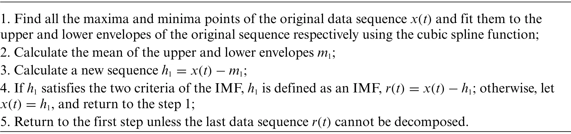
Table 1: EMD algorithm

The EMD method has been applied quickly and effectively in different engineering fields,such as in oceans,atmosphere,celestial observations and geophysical record analysis.But an inevitable shortcoming of EMD,mode mixing which is caused by the data intermittency,such as intermittent signal,impulse interference and noise,limits its application.Mode mixing refers to an IMF containing extremely different characteristic scales or similar characteristic scales distributed in different IMFs,causing adjacent IMFs to mix together.

Aiming at this phenomenon,Huang proposed the EEMD which use Gaussian white noise in original sequence.When the signal is added to a uniformly distributed white noise background,signal regions of different scales are automatically mapped to the appropriate scale associated with the background white noise.Due to the characteristics of zero-mean noise,the noise will be canceled after multiple averaging calculations.

The steps of EEMD algorithm steps are shown in Table 2.

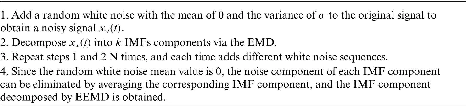
Table 2: EEMD algorithm

2.2 Autoregressive Integrated Moving Average(ARMA)

The ARMA model is mostly used in time series forecasting.For a given data set of ship motion

where p and q are the model order of the AR and MA,respectively.εtis a white noise with finite variance,αpandβqare the regression coefficients of the ARMA model.The most important step in model construction is to determine the model orders p and q,which are generally identified by autocorrelation functions and partial autocorrelation functions.In order to fit the data as much as possible and avoid overfitting,Akaike Information Criteria(AIC)was used for model identification in this paper.

where k is the number of parameters,Lis the likelihood:

wherexiis the observed,andis the prediction,(xi-)is the prediction residual.In the model identification,the AIC value is minimized,which determines the smallest appropriate order to represent the time series.

2.3 Back Propagation Neural Network(BPNN)

Artificial neural networks have been widely used in recent years to construct time series prediction models because they can fit functions of arbitrary complexity with arbitrary precision.As a classic algorithm,BP network is favored by many researchers.A typical predictive network structure with one input layer,one hidden layer and one output layer is as follows:

In general,the output of the neural network is

wherepandnare the number of input layer and hidden layer neurons,respectively.wih,who,bh,boare the coefficients of the input layer and the hidden layer,coefficients of the hidden layer and output layer,offsets of the hidden layer and output layer,respectively.fhandfoare the hidden layer activation function and output layer activation function,respectively.A network structure with one input layer,two hidden layers and one output layer is adopted in this paper.

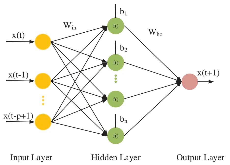
Figure 2:The structure of BPNN

2.4 Support Vector Regression

For a given training setT={(x1,y1),(x2,y2),...,(xN,yN)}

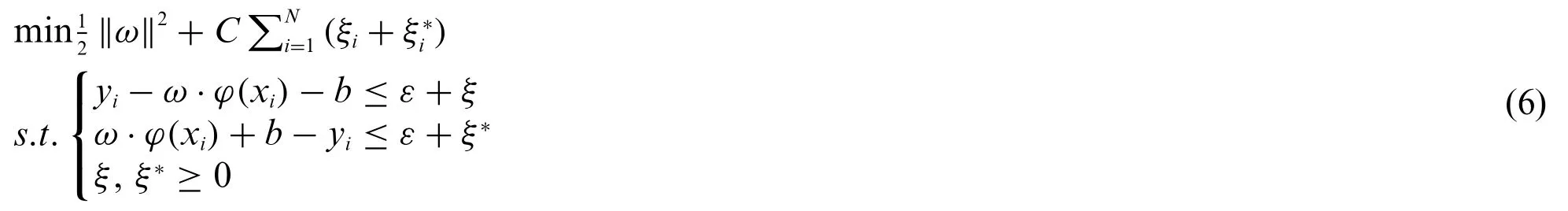
wherexi∈Rnis n-dimensional input of the ship motion,yi∈Ris the prediction value,the aim of SVR is to find a hyperplane that fits y without errors under the given accuracyε,that is,the distance from all sample points to the optimal hyperplane is not greater thanε.SVR tries to map initial data from the sample space into a higher dimensional feature spaceRmthrough a nonlinear mapping function and thus converts a nonlinear problem into linear problem to get the optimal solution.The SVR model is constructed as follows:

whereφ(x)is the nonlinear mapping function,ωis the weight vector,b∈Ris the threshold,“·”is the dot-product in the feature space.Taking into account the allowable error,we introduce slack variablesξ,ξ*and penalty parameterC,therefore transform the above problem to a convex optimization problem:

After converting the optimization problem into a dual problem,the optimal regression function can be solved as

whereαiandare the Lagrange multipliers,K(xi,x)=φ(xi)·φ(x)is the kernel function,and gaussian function is choose as the kernel function in the paper.

2.5 Ensemble Trees

Decision tree is a well-known predictive model with many advantages such as intelligibility and small amount of computation,therefore,it is widely used in data science and competition.But a simple regression tree has the disadvantage of easily fitting the training data and unstable,therefore,little change in training data may result in very different trees and predictions.Ensemble trees are one solution to improve robustness and reliability of regression trees by combining multiple regression trees produced with different generation methods.RF and XGBoost are two widely used ensemble models but with different features.

The RF first randomly samples the original sample set by the Bootstrap sampling method to obtaintsamples containingmsamples,so that 63.2%of the samples in the initial training set appear in all sampling sets.Based on each sample set,a regression tree can be built.The process of RF regression tree is different from the traditional decision tree.It randomly extractskfeatures from all features as the split feature set of the current node.Each regression tree grows from top to bottom recursively,and all decision trees are combined.Random forests.The final predicted result is the average of thetregression trees predictions.

XGBoost is a scalable end-to-end tree boosting system,which is used widely by data scientists to achieve state-of-the-art results on many machines learning challenges.The goal of this model is to predict the outputywith inputx,

whereKis the number of the functions,Γ represents a set of regression functions.

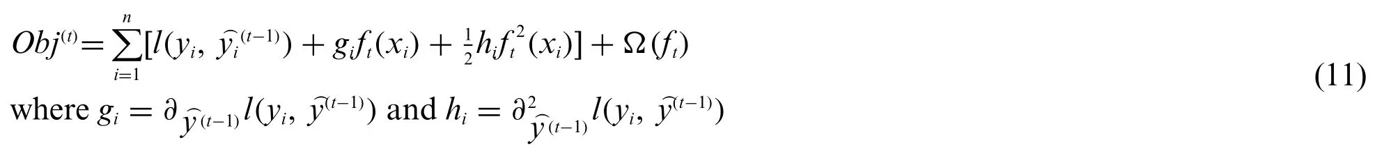
The objective function of XGBoost is as follows:

wherelis the loss function indicating the difference between the prediction ^yiand the targetyi.Ω is the complexity of a single tree including the number of leavesTand the regular term of the residualωto prevent overfitting.

During the training process,the training objective function of each tree is shown in

The second-order Taylor expansion of the objective function is

fis defined as

whereqis a structure function that maps inputxto the index of the lead node.wgives the leaf score corresponding to each index number.

Iis defined as a sample set above each leaf:

therefore,

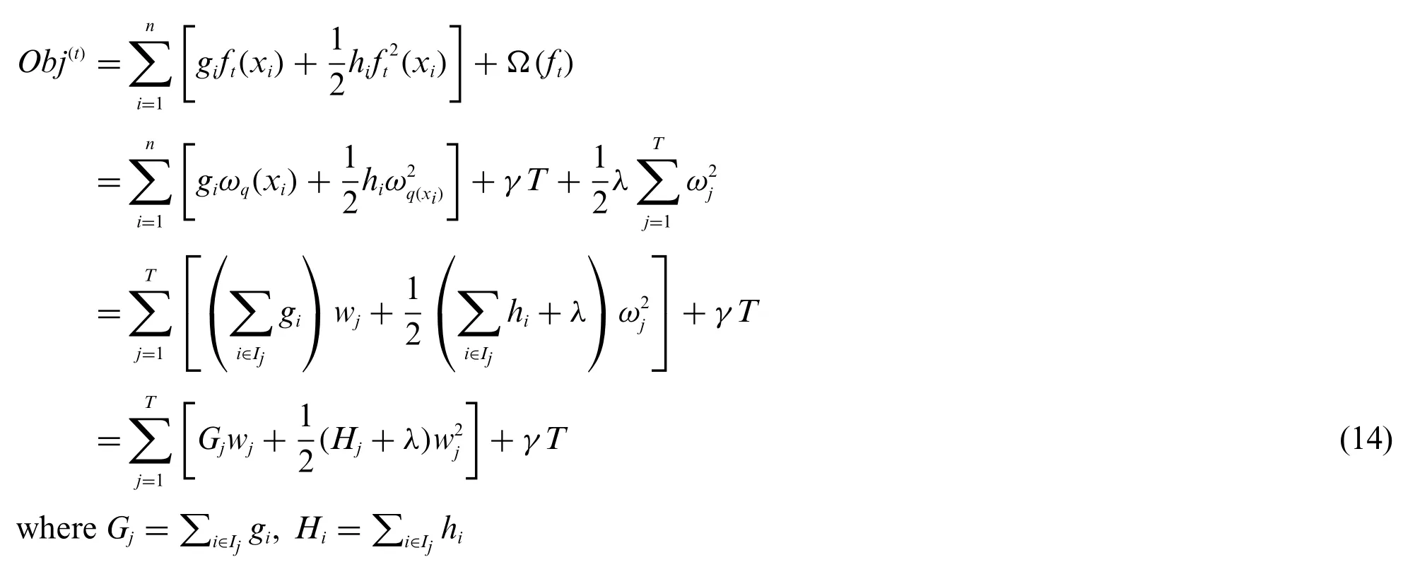
Then the optimalcan be obtained as follows:

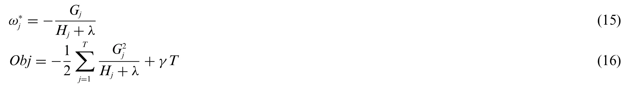
The good structure can be obtained by the objective function.In order to balance the new node complexity and objective function,exact greedy algorithm was adopted by the authors to calculate the gain in the loss reduction from introducing the split:

L,Rrepresents the left and right nodes of the leaf.

2.6 Genetic Algorithm

Genetic algorithm is a randomized search algorithm generated by evolutionary theory and genetic mechanism,which adaptively adjust the search direction and can be used to optimize parameters without falling into the local optimal solution.Genetic algorithms mainly include chromosome coding,evaluation of fitness,selection,and hybrid mutation operations.In the paper,the GA algorithm is used to optimize the two parameters of the RF prediction model,which are the maximum depth of the tree and the number of base classifiers.First,set the range of values for the two parameters,it determines the required number of binary coded,which map the parameter space into to the chromosomal space.An initial binary coded chromosome of a certain size is then randomly generated,and fitness of each individual in the initial chromosome population is calculated.Roulette wheel selection,deterministic or tournament selection are adopted to select individuals with higher fitness values from the group they have higher opportunity to transmit the good genes to the next generation as parents.Then the core operational variations and intersections in the genetic algorithm are executed,improving the search ability of the genetic algorithm and promoting the group to continuously develop toward the optimal solution.Fig.3 shows the algorithm structure of EEMD-GARF.

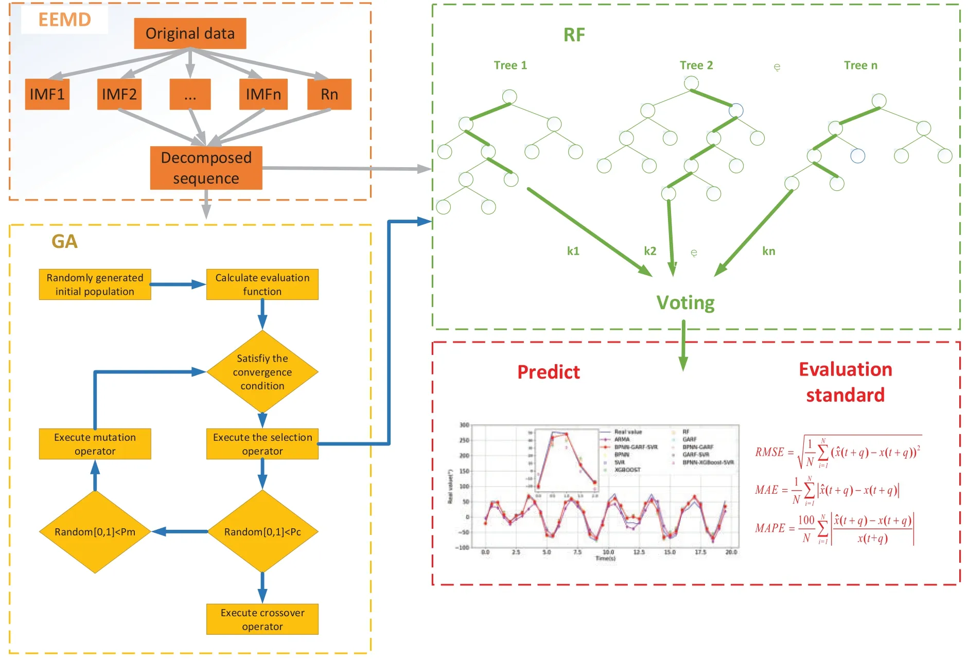
Figure 3:The framework of the EEMD-GARF model

2.7 Combined Prediction Based on Correlation Coefficient

In order to reduce the risk of prediction,a combined forecasting method came into being,the most concerned issue of which is how to find the weighted average coefficient.In most cases,the timevarying weight combination method produces better results than the constant weight combination method.A combined prediction model based on correlation coefficients is adopted in this paper,and the optimal solution of weighting coefficients is determined by the error square sum criterion.

We assume the observations are {xt,t=1,2,...,N},the predicted values of the prediction models are

where m is the number of the model.Combined forecast value is as follows:

liis the weight coefficient of thei-th prediction method.

The correlation coefficient between the predicted sequence of thei-th single prediction method and the actual observed sequence is

The correlation coefficient between the combined predicted value and the actual observed value is

whereet=xt-

We define

Then the(21)can be obtained

Eijrepresents the covariance of the predicted values of thei-th andj-th prediction methods,andEijrepresents the variance of the predicted value sequence of thei-th method.Eis the covariance information matrix of the combined prediction.

It is obvious that the largerRis,the more effective the prediction method is,so the solution of the weighting coefficient can be defined as an optimization problem as follows:

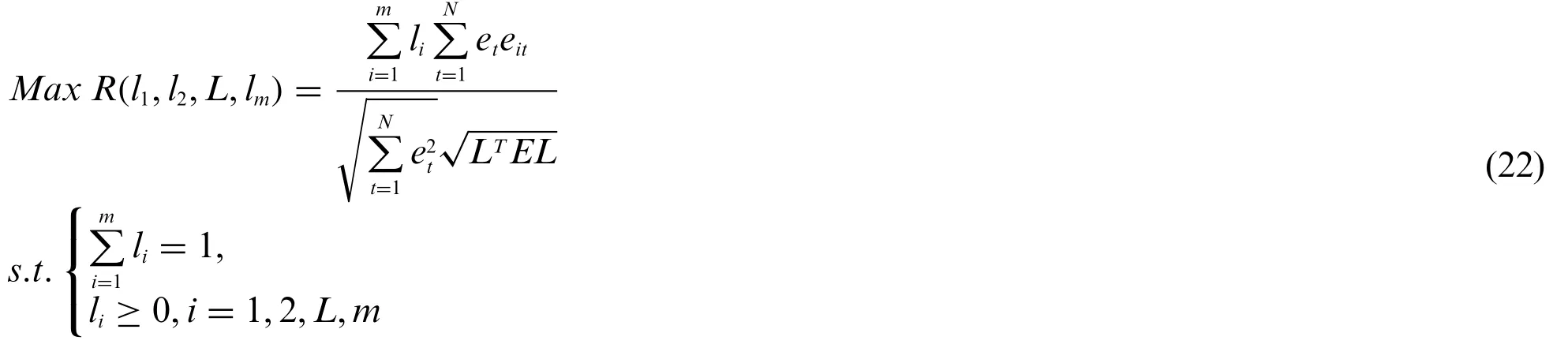
WhenRis the largest,thelis the weight coefficient of each model.When the optimal solution has more than two components that are not zero,that is,two or more single prediction methods provide effective information,the combined prediction method corresponding to the optimal solution is better than the best one of the single prediction methods.

3 Result and Experiment

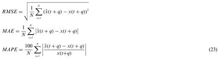
In the paper,ARMA,BPNN,SVR,RF,GARF,XGBOOST are selected as the single prediction model to forecast the ship motion and BPNN-GARF,GARF-SVR,BPNN-XGBoost-SVR and BPNN-GARF-SVR are designed as the hybrid models.The data used in this paper is the measured data of the ship sailing in the sea,whose sampling frequency is 10 Hz.Three common criteria,root mean square error(RMSE),the mean absolute deviation(MAE)and the mean absolute percentage error(MAPE)were adopted to measure the prediction performances of the models.The definition of the RMSE,MAE,MAPE are as follows:

For the model mentioned in the article,parameter adjustment is very important,which helps to improve the prediction accuracy of the model.The parameters of used models were set and determined as the following.For ARMA model,orders p and q were determined by Akaike Information Criterion(AIC)with the coefficientsαandεwere calculated by recursive least square method.The decomposition parameters of EEMD are set according to common settings whereσ=0.1,N=100.In the BPNN model,the parameters with better performances are adopted as the number of neurons.Therefore,a BPNN structure containing an input layer,two hidden layers,and an output layer is designed in the text,where the number of neurons is 100,10,10,100,respectively.The weight coefficients and offset coefficients between the layers are first randomly initialized and then optimized by the gradient descent method.The Gaussian function is used as the kernel function in the SVR model.The XGBoost use a grid search method to determine multiple parameters.In the GARF model,the range of values of the two parameters are taken as[10,160]and[1,64]and intervals are 10 and 1,respectively,therefore,the number of coded bits is 10 bits.The number of populations and the number of iterations is both set to 50,the mean square error of predicted and true values is adopted as the fitness function of the model.

A set of 100 s with a sampling frequency of 10 Hz is created for EEMD decomposition and the Fig.4 is the result of EEMD.The ship motion series is divided into 8 IMFs and one residual.The original sequence is divided into 8 IMFs and one residual,and all IMFs are arranged in the order in which they are extracted,with frequencies from high to low.It can be seen from the decomposition results that the original sequence is mainly controlled by low frequency sequences such as IMF2,IMF3,and IMF4.In all IMFs,the IMF1 with the highest frequency is considered as noise,and the remaining IMFs and residuals are re-added into a new approximate sequence,the complexity of which is reduced.

The Fig.5 shows the instantaneous frequency of each IMF sequence.The fold lines are IMF1～IMF5 from top to bottom,and the frequency is also from high to low,which is consistent with the decomposition result of the Fig.5.It can be seen that the main IMFs are clearly separated into different frequency components and there is no mode mixing.

This paper used 0.1 s as the initial prediction step,and each prediction is increased by 0.1 s until 9.9 s.The Fig.5 describes the true value and the predicted value curve for the 50-step prediction of different models.The Table 3 shows the prediction accuracy of the 10 prediction models from the three evaluation criteria RMSE,MAE,MAPE when predicting 50 steps.

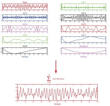
Figure 4:EEMD decomposition results and reconstruction sequences

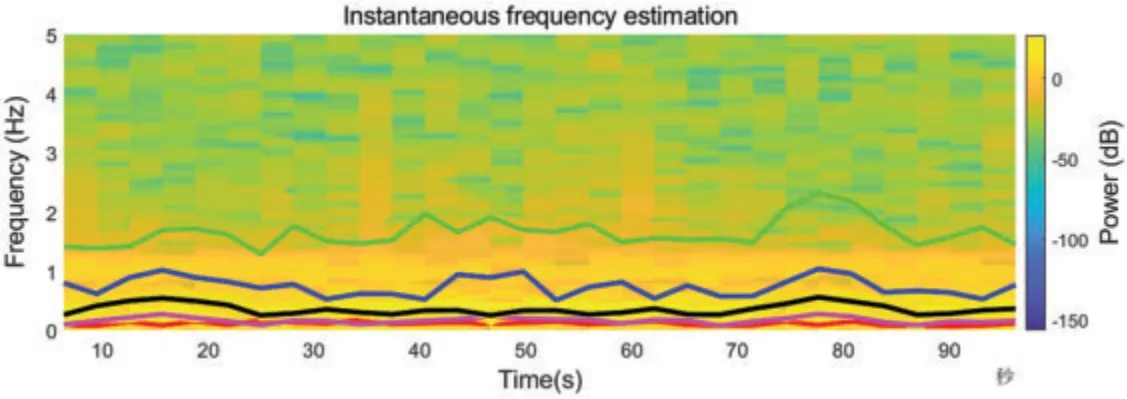
Figure 5:Instantaneous frequency estimation of the IMFs

As can be seen from the Fig.6 and Table 3,as a linear model which is easy to construct,the prediction accuracy of ARMA model is inferior to all other models when it is used to predict the complex nonlinear ship motion.As a model with strong nonlinear fitting ability,BPNN and XGBoost models behave much better than ARMA model,but they are inferior to SVR and RF models in a single model.The RF model optimized by the genetic algorithm has better performance,but the improvement effect brought by the genetic algorithm cannot make the RF model exceed the SVR model,whose performance is the best in the single model when predicting 50 steps,and the RMSE,MAE,MAPE of which is 10.26,7.47,0.91.

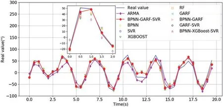
Figure 6:Ship motion prediction curve for all models

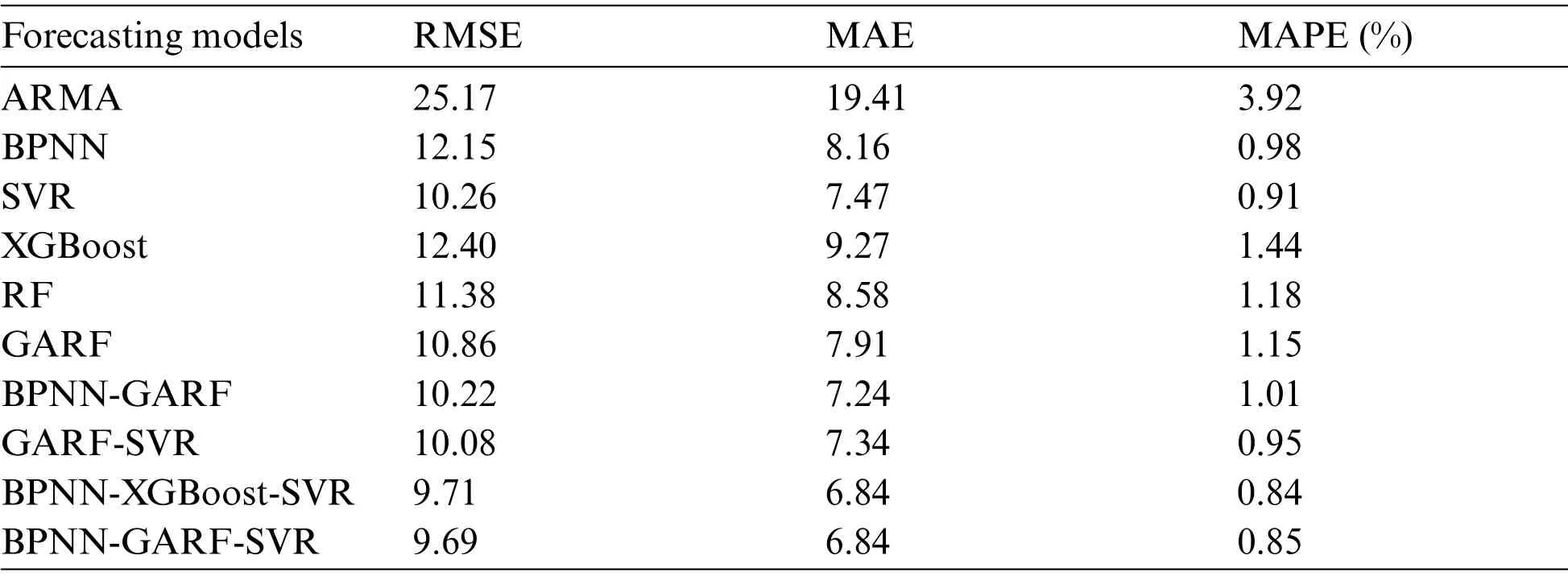
Table 3: Prediction accuracy of each model when the forecast step is 50

Among the four combined models used in the article,BPNN-GARF has similar performance with SVR while the other three models GARF-SVR,BPNN-GARF-SVR,BPNN-XGBoost-SVR have higher precision than the SVR model,which indicates the prediction method designed in the paper is at least non-inferior combination.GARF-SVR can be regarded as a redundant combination forecast model because compared to the SVR model(RMSE=10.26,MAE=7.46,MAPE=0.91)and the GARF model (RMSE = 10.87,MAE = 7.91,MAPE = 1.15),three evaluation criteria of GARFSVR model(RMSE=10.08,MAE=7.34,MAPE=0.95)only increased by 0.18,0.12,-0.04(1.7%,1.7%,-5%)and 0.79,0.57,0.20(7.3%,7.2%,1.7%),respectively.The RMSE and MAE criteria only increased by less than 2%compared with the SVR,and the MAPE even decreased by 5%.

From the Fig.5,it can be seen that the combined prediction results in the GARF-SVR mainly depend on the SVR,and the weight coefficient of GARF,which cannot provide much useful information for the final forecast result,is only 0.25 while the coefficient of SVR is 0.75.BPNN-GARF is a typical superior combination model.Compared with BPNN and GARF,the performance of BPNN-GARF(RMSE=10.22,MAE=7.24,MAPE=1.01)is increased by 1.94,0.09,-0.03(16.0%,11.3%,-3.0%) and 0.65,0.68,0.14 (6.0%,8.6%,1.3%),respectively,at least to the extent of SVR.BPNN-GARF combination model can be depicted as an excellent combination that achieve better results than a single model by combining a better model with a poorer model.The other two combined models BPNN-GARF-SVR and BPNN-XGBoost-SVR are basically similar in performance,because the most useful information of these two models is contributed from SVR,and GARF and XGBoost only provide a little effective information,which can be seen from the weighting coefficients.In the BPNN-GARF-SVR combination model,the weight coefficients of BPNN,GARF,and SVR are 0.30,0.18,and 0.52,which are the same as the BPNN,XGBoost,and SVR weight coefficient bases in the BPNN-GARF-SVR model,0.32,0.09,and 0.59.Since XGBoost is inferior to GARF,the latter has a higher weighting coefficient than the former.Compared with the SVR model,the BPNN-GARFSVR model has improved by 0.57,0.63,0.53,(5.5%,8.4%,5.9%).For the BPNN and GARF models,the improvement of the combined model is more obvious that the performance is increased by-2.46,-1.32,-0.12%(20.2%,16.1%,12.2%)and-1.17,-1.078,-0.29(10.8%,13.6%,25.6%),respectively.From the above conclusions,by combining a plurality of individual prediction models,an integrated model with better performance can be obtained.

Figs.7a–7c show the relationship between prediction accuracy and prediction step size.It can be observed that when the prediction step size is less than 10,the BPNN effect is the best an as the prediction step size increases,the SVR and GARF models gradually achieve better results.GARF model is significantly better than RF,but the optimization effect gradually decreases with time.This is because the genetic algorithm optimization result is adopted as a fixed parameter for RF model which does not change with the prediction step size increases.The prediction result curve from GARF-SVR also concludes that this is a redundant prediction model because the performance curve of GARFSVR almost coincides with the curve of SVR.

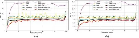
Figure 7: (Continued)

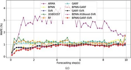
Figure 7:The curve of prediction accuracy and forecast step size

In the BPNN-GARF/XGBoost-SVR model,the performance is always superior to the current single prediction model.When the prediction step is small,BPNN is better than SVR and GARF and the combined model is better than BPNN.With the increase of the prediction step size,SVR is better than BPNN and GARF,and the combined prediction model is superior to SVR.Compared to BPNN and SVR,GARF and XGBoost have small weight coefficients in combined forecasting,but they also provide some useful information to the final result.

The Fig.8 shows the variation of the weight coefficient with the predicted step size.At the beginning,BPNN’s weight coefficient is the highest,then gradually decreases and tends to stabilize,while the SVR coefficient is gradually increasing.The coefficient of GARF is relatively low,and sometimes close to zero.Therefore,SVR provides the main valid information,BPNN provides secondary useful information,and GARF also provides useful information,but sometimes it may be redundant.

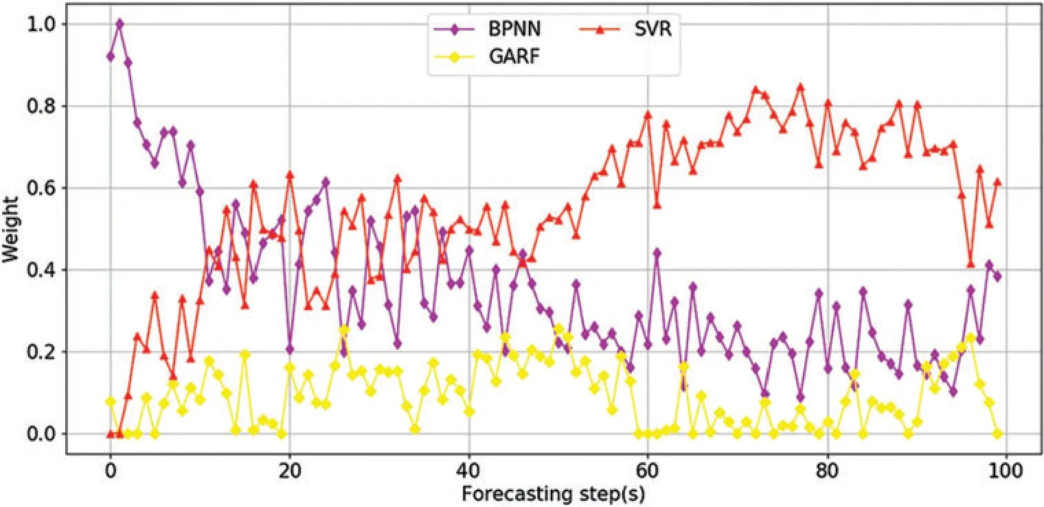
Figure 8:The curve of BPNN-GARF-SVR weight coefficients and forecast step size

The Fig.9 shows the correlation coefficient between the predicted value and the real value,which provides another perspective for evaluating the performance of the model,and the weight coefficient in the combined model is also determined according to the correlation coefficient of each single model.The correlation coefficient of the combined model is obviously higher than the single model,which is consistent with the results of three evaluation criteria.

The Figs.10a–10d show the correlation coefficients of BP,GARF,SVR and BPGARF when predicting 50 steps.The correlation coefficient of the combined model is higher than the correlation coefficient of the single model,which is consistent with the previous analysis.

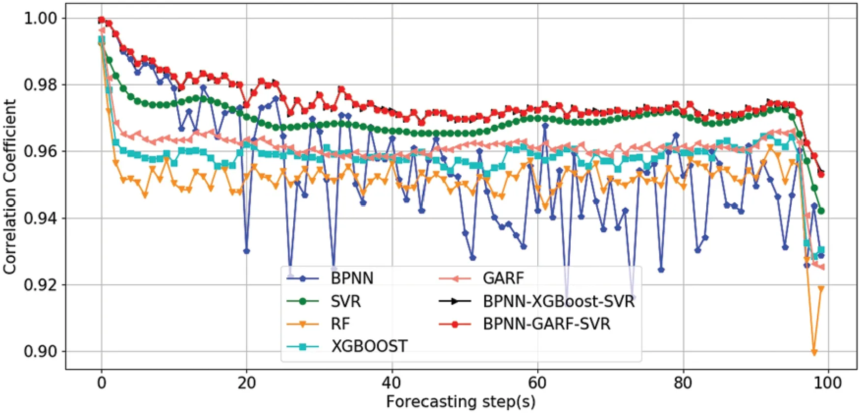
Figure 9:The curve of correlation coefficient and forecast step size

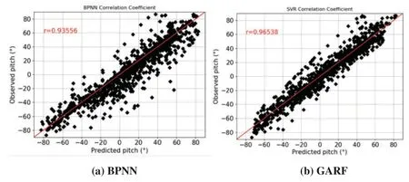
Figure 10: (Continued)

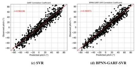
Figure 10: The correlation coefficient of the BPNN,GARF,SVR and BPNN-GARF-SVR when forecast step is 50

4 Conclusion

In this paper,we proposed a hybrid forecasting method EEMD-BPNN-GARF-SVR for ship motion.EEMD is used to remove high frequency noise components from the original sequence and obtain reconstructed sequences.Three independent predictive models were first established based on the reconstructed data,including BPNN,SVR and RF models.The final prediction results are obtained by combining the prediction results of three independent prediction models.Experiments show that for the measured data,when the prediction compensation is 50 steps,the RMSE,MAE and MAPE of the BPNN-GARF-SVR model are 9.69,6.84 and 0.85,respectively.The RMSE of the single models is greater than 10,the MAE is greater than 8,and the MAPE is greater than 1.It can be seen that through the combination of multiple models,the prediction result is improved compared to the single prediction model.

Funding Statement:The authors received no specific funding for this study.

Conflicts of Interest:The authors declare that they have no conflicts of interest to report regarding the present study.