Finite Element Simulation of Radial Tire Building and Shaping Processes Using an Elasto-Viscoplastic Model

Yinlong Wang,Zhao Li,Ziran Li,⋆and Yang Wang

1Department of Modern Mechanics,CAS Key Laboratory of Mechanical Behavior and Design of Materials,University of Science and Technology of China,Hefei,230027,China

2Wuhan Second Ship Design and Research Institute,Wuhan,430064,China

ABSTRACT The comprehensive tire building and shaping processes are investigated through the finite element method(FEM)in this article.The mechanical properties of the uncured rubber from different tire components are investigated through cyclic loading-unloading experiments under different strain rates.Based on the experiments,an elastoviscoplastic constitutive model is adopted to describe the mechanical behaviors of the uncured rubber.The distinct mechanical properties,including the stress level,hysteresis and residual strain,of the uncured rubber can all be well characterized.The whole tire building process(including component winding,rubber bladder inflation,component stitching and carcass band folding-back)and the shaping process are simulated using this constitutive model.The simulated green tire profile is in good agreement with the actual profile obtained through 3D scanning.The deformation and stress of the rubber components and the cord reinforcements during production can be obtained from the FE simulation,which is helpful for judging the rationality of the tire construction design.Finally,the influence of the parameter “drum width” is investigated,and the simulated result is found to be consistent with the experimental observations,which verifies the effectiveness of the simulation.The established simulation strategy provides some guiding significance for the improvement of tire design parameters and the elimination of tire production defects.

KEYWORDS Uncured rubber;constitutive modeling;radial tire;building process;finite element method

1 Introduction

Tires are one of the most important components of vehicles such as automobiles and airplanes.A high-quality tire will be quite durable,and can greatly enhance the driving experience.To produce a tire,the semifinished parts are first produced through a calendaring or extrusion process.Then,all these components go through stitching and assembling processes(including component winding,rubber bladder inflation,component stitching and carcass band folding-back)to form the final green tire.This completes the tire building process.Next,the green tire is put into a curing mold and expanded inside the mold to adopt its shape under high-pressure and high-temperature.A finished tire with a complex and unique tread pattern is eventually formed.This completes the tire shaping process.In production,tire building and shaping are quite important and complex processes where the component deformation and the stress distribution are very complicated.It is believed that most production defects in the finished tire initially appear in these two processes.

During tire production,the deformation and stress distribution of some components may have a great influence on the final performance of a finished tire.For example,the cord reinforcements embedded in rubber are the main load-bearing components of tires [1,2],and the layup of the cord reinforcements would significantly influence the tire carrying capacity [3–5].However,during the tire building and shaping processes,the layup of the cord plies could change significantly with the deformation of rubber components and may deviate from the design specifications,resulting in a production defect(cord twisting,shoulder flection and so on).Usually,the trial and error method is used to determine the cause of this kind of production defect,but this method is quite costly and timeconsuming.In recent years,with the improvement of finite element simulation technology,studying tire production using simulation methods could be a better choice to eliminate some tire production defects by improving the tire design parameters.

To carry out the finite element simulation on tire production processes,the first thing that needs to be addressed is the characterization of the mechanical behaviors of the uncured rubber,which is in a processing state and has quite different mechanical properties compared to cured rubber[6,7].In recent years,the mechanical properties of uncured rubber have been reported by several investigators[8–14].They conducted viscous types of material tests and found that the mechanical properties of uncured rubber are highly rate-dependent.Nonlinear elastic-inelastic behaviors involving stronger hysteresis and shape recovery can be clearly observed under cyclic loading conditions.However,despite the differences in the elastic and viscoplastic level,the uncured rubber and cured rubber are both elastoviscoplastic polymers.And some well-developed constitutive models for cured rubber,such as the generalized Maxwell model[15],the extended eight-chain models[16,17],and the recently developed hyper-visco-pseudo-elastic models[18–21],can provide instructional significance for the mechanical property characterization of the uncured rubber.Kaliske et al.[8]first proposed a phenomenological constitutive model based on the linear viscoelasticity framework to describe the nonlinear mechanical behaviors of the uncured rubber.This framework is a rather simple construction with respect to the nonlinear response.Later,a microsphere-based viscoplastic constitutive model[14],which consists of a rate-independent part and a rate-dependent part,and a neural network-based approach[10],which has an advantage of numerical efficiency,were proposed to improve the characterization capabilities.However,the rate-dependent plastic deformation behaviors of the uncured rubber still didn’t get well characterized.Recently,Li et al.[11]carried out detailed experiments,including the monotonic tensile tests,cyclic loading tests and relaxation tests,on uncured rubber and proposed an elasto-viscoplastic constitutive model based on the molecular network.This constitutive model,which includes the nonlinear viscous flow and the Mullins effect,can better characterize the complex mechanical behaviors of uncured rubber,but has not been applied to the simulation of actual production process.

To date,the simulation method has been used for tires to analyze tire deformation,stress,strain,tire rolling and tire dynamics over a long period and has yielded many useful achievements [22–25].However,the tire building process,which directly determines the final performance of a tire,has not been well studied.Wang et al.[26,27] used the finite element method for the first time to simulate the entire building process of a wide-based radial truck tire.Based on the simulation results,they put forward some strategies to reduce and eliminate some tire production defects.However,in these simulations,the adopted constitutive model based on the Marlow spring and Maxwell elements may be a somewhat simple construction with respect to the highly nonlinear mechanical responses of the uncured rubber.On the other hand,the finite element models and the simulation processes have been greatly simplified.For example,the component winding process was simplified compared to practical production,and several structural components of the building machine were neglected.These simplifications may reduce the reliability of the simulation results directly.Compared to the tire building process,the tire shaping process,which is widely considered to be the most important process in tire production,has received much more attention over the years.Most of these studies focus on the state-of-cure(SOC)of the rubber material during the curing process and try to find the optimum curing time and pressure to achieve the optimal performance of the finished tire [28–32].However,the deformation of rubber materials and cord reinforcements during the shaping process has not been extensively investigated.To observe the flow of tread rubber during the shaping process,Choi et al.[33]conducted a tire shaping experiment with white rubber strips inserted inside the black tread rubber,and the corresponding simulation was in good agreement with the experiment.However,the other components were not simultaneously investigated,and the cord reinforcements were also not discussed.During the initial stage(1 to 2 min)of the shaping process,the rubber material can quickly fill the mold under a high-pressure environment.While the SOC of the tire is still very low,most of the rubber materials remain uncured except for a few surface areas[30].Hence,simulating the early tire shaping process through FEM without considering the changes in the physical properties of rubber materials is a reasonable and meaningful method to investigate the mechanical behaviors of rubber materials and cord reinforcements.

In this paper,the FEM is used to study the building and shaping processes of all-steel radial truck tires.Uniaxial tensile experiments for rubber compounds from different components were first conducted at different strain rates.Then,a nonlinear elasto-viscoplastic constitutive model was presented to fully describe the mechanical behaviors,including the hypothesis and the residual strain of the uncured rubber,and the calibration results were depicted.On this basis,finite element models of different tire components were established,and the fully green tire building process and the tire shaping process under high pressure were simulated.The simulation flow and techniques were refined to make the simulation results more consistent with reality.The mechanical behaviors of the rubber components and the embedded cord reinforcements can all be obtained from the FE modeling result.The simulated green tire profile was compared with the actual green tire profile obtained by 3D scanning,and it was found that the two profiles overlapped well.Finally,the influence of the parameter“drum width”was investigated to provide some guiding significance for the improvement of tire design parameters.

2 Experiment and Modeling of Uncured Rubber

2.1 Experiment

The rubber compounds from different tire components were provided by Giti Tire,Ltd,(Singapore).Sulfur is not contained to prevent polymer chain crosslinking during the specimen preparation process.This does not influence the material behaviors of the uncured rubber.

The specimen used in the experiments is a dumbbell whose shape and size (in millimeters) are shown in Fig.1a.The thickness is 3 mm.For soft materials such as rubber,the end effect during tensile experiments often causes larger strain measurement errors.Here,a noncontact strain measurement method,namely,the automatic grid method[34,35],was used to eliminate the errors.The grid array was installed on the specimen surface to record the strain field information of the specimen during the tensile process,as shown in Fig.1b.Detailed descriptions of the test system and specimen preparation process are given in our previous reports[11].

Figure 1: The uncured rubber specimen (a) Tensile test specimen (b) The uncured rubber specimen disposed with white grid array

The tensile behaviors of the uncured rubber were evaluated through uniaxial cyclic loading tests at different strain rates(0.001/s,0.003/s,0.03/s and 0.1/s)under room temperature.The cyclic loading tests,which include hysteresis and residual strain during the loading processes,can accurately reflect the elasticity level,viscosity and plasticity of the uncured rubber.Each test was carried out on three different specimens to ensure the reliability of the experimental results.

The experiments are controlled by strain,and each test includes four loading and unloading cycles with increasing strain values(0.2,0.4,0.6 and 0.8).The investigated tire contains 15 different rubber compounds.To save space,only two rubber compound experiments(tread rubber and sidewall rubber)are presented here.The test results are depicted in Fig.2.The figure shows that the two rubber compounds have similar mechanical characteristics,including a distinct hysteresis effect,residual strain and rate dependence.The tread rubber has relatively higher elasticity and viscosity,and they are slightly lower for the sidewall rubber.For both rubber compounds,the tensile stiffness decreases with increasing strain during every loading step,and the hysteresis loops that represent the viscosity are quite noticeable.The rate-dependence of the uncured rubber during the tensile process is quite significant.With increasing stain rate,the stress level clearly increases,and the residual strain,which reflects the viscoplasticity,deceases;that is,the elasticity intensifies,and the viscoplasticity weakens.To show the changes in the elastic behaviors more clearly,the stress-strain curves of the tread rubber over the first 20%strain range of every loading cycle were fitted by the linear elastic model,as shown in Fig.3a.It can be seen that the elastic modulus increases with the increasing strain rate,and decreases with the increasing number of loading cycles.The decrease in the elastic modulus,which usually occurs in the first loading cycles for elastomers,is referred to as the“Mullins effect”[36,37].Fig.3b shows the residual strain variation of the tread rubber with the increasing number of cycles under different strain rates.And the decrease in the viscoplasticity with increasing stain rate can be clearly observed.

Figure 2:Cyclic loading–unloading tensile tests

Figure 3:Variations in the elastic modulus and residual strain with the increasing number of loading cycles under different strain rates

2.2 Modeling of Uncured Rubber

As mentioned in the previous section,the mechanical properties of uncured rubber,which involve elasticity,viscosity and plasticity,are quite complicated.Here,to properly characterize the constitutive behaviors of the uncured rubber,an elasto-viscoplastic constitutive model based on the eight-chain model [38] and Bergstrom-Boyce flow [39,40] is adopted.The constitutive model is based on the three networks interpretation,which decomposes the rubber network into a carbon black filled chain network(Hyperelastic network A)and two free chain networks that are composed of entangled free chains(Elastic-viscoplastic network B)and nonentangled free chains(Elastic-viscoplastic network C),as shown in Fig.4.

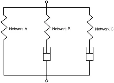
Figure 4:The parallel network model

Based on the eight-chain model,the Cauchy stresses for the three networks can be written as:

whereμis the shear modulus,Lis the Langevin function,L(x)=cothx−1/x,Nis the average number of“rigid links”between two molecular joints,B is the left Cauchy-Green tensor,B=FFT,B∗is the distortional part of B,B∗=J−2/3B,anddevB∗is the deviatoric part of B∗,devB∗=B∗−are the effective chain stretches for three different networks,λchain=where C is the right Cauchy-Green tensor,andλ1,λ2,λ3are the principal stretches.The derivation process is shown in Appendix A.

For elastic-viscoplastic networks (Networks B and C),the total deformation gradient can be multiplicatively decomposed into elastic and viscoplastic parts [41],F=FBeFBvand F=FCeFCv.The elastic parts of the deformation gradient provide the Cauchy stress,and the viscoplastic parts contribute to the viscoplastic deformation.

The viscoplasticity of the uncured rubber has been illustrated in the previous section.The viscoplastic residual strain accumulates gradually with the deformation process,and the increasing strain rate can decrease the visoplasticity level.For this complex mechanical behavior,the general Maxwell element is not sufficient for accurate characterization.Here,the Bergström-Boyce flow model[39,41],which is based on the reptation of macromolecules[42],is adopted to model this timedependent mechanical behavior.According to this model,the rate of viscoplastic deformation in the two networks can be constitutively prescribed as follows:

Then,the viscous parts of the deformation gradients,FBvand FCv,can be integrally derived [40].The elastic parts of the deformation gradients are obtained:

Moreover,for uncured rubber,the “Mullins effect”,can be clearly observed during tensile processes.To describe the Mullins softening effect of the uncured rubber,the Ogden-Roxburgh Mullins Effect model[43]is adopted in the elastic components in Network B and Network C.It is written as:

whereηis the damage variable that evolves with the strain energy,η=1−where[r,α,]are material parameters,erf (x)is the error function,Ucuris the current strain energy density.Following the eight-chain model,it is written as:

wherenis the average chain density (number of molecular chains per unit reference volume),β=is the current elastic effective chain stretch,kBis Boltzmann’s constant,andΘis the reference temperature.Umaxis the state variable for the evolving maximum strain energy density at the material point in its deformation history:

whereβ=is the evolving maximum elastic effective chain stretch.

Plugging Eqs.(2)and(3)into Eq.(7),the Cauchy stresses for the two elastic-viscoplastic networks are finally obtained.

The three stresses can be added to obtain the total Cauchy stress:

2.2.1 Computation of the Algorithmic Tangent Stiffness Matrix

For the implicit analysis in a finite element simulation,the tangent stiffness matrix of the constitutive model needs to be derived.However,for the constitutive model in this paper,a closed-form continuum tangent stiffness matrix is quite difficult to obtain.Here,a feasible and simple numerical calculation method of an approximated algorithmic tangent matrix was adopted[44].

The numerical calculation strategy,which is based on a perturbation technique,can be written as:

whereΔσ(Δε)is the stress increment tensor,Δεis the strain increment tensor,δis a small perturbation parameter(<<||Δε||),andδεis an“almost zero”tensor.

The constitutive model in this paper is developed based on the deformation gradient.Following the perturbation technique,the perturbation of the deformation gradient F is produced by perturbing only its componentsF(i,j)andF(j,i)(i,j=1,2,3).Here,we denoteΔF(ij)as the perturbation to the deformation gradient produced by perturbing only it(i,j)and(j,i)components:

where the choice of“ij”would be“11”–“13”,“22”,“23”and“33”,F is the total deformation gradient,{ei}i=1,2,3is the base vector in the spatial configuration.

The perturbed total deformation gradient,,can be expressed as:

Substituting Eq.(13) into Eq.(6),the perturbed elastic parts of the deformation gradients for Networks B and C can also be obtained:

Using the perturbed deformation gradient,the perturbed Cauchy stress can be calculated based on the constitutive equation:

Combining Eqs.(10)and(15),the Eq.(11)can be written as:

where six independent components of C(ij)are determined by the perturbation ofΔF(ij).The tangent stiffness matrix C has a total of 36 components.Hence,after the six perturbations ofΔF(ij),all the components of C can be obtained.

2.2.2 Model Validation

To verify the reliability of the constitutive model,the model was used to fit the cyclic loading tests for two rubber compounds.The fitting method can be written in the form of a mathematical minimization problem.

whereσpredis the predicted stress vector,σexpis the experimentally determined stress vector,andNis the number of experimental datasets.The Monte Carlo method[45]was used to give an initial guess of the material parameters.The normalized mean absolute difference method was applied to obtain the optimal material parameter values and the gradient descent method was adopted for the optimization process.The calibration results were depicted in Fig.5.It can be observed from the figure that the modeling curves fit the experimental results well and the stress and deformation characteristics(stress level,hysteresis,residual strain and the rate-dependence)can all be properly described for two rubber compounds.The optimization parameters are shown in Table 1.To save space,only the parameters for the tread rubber are given here.

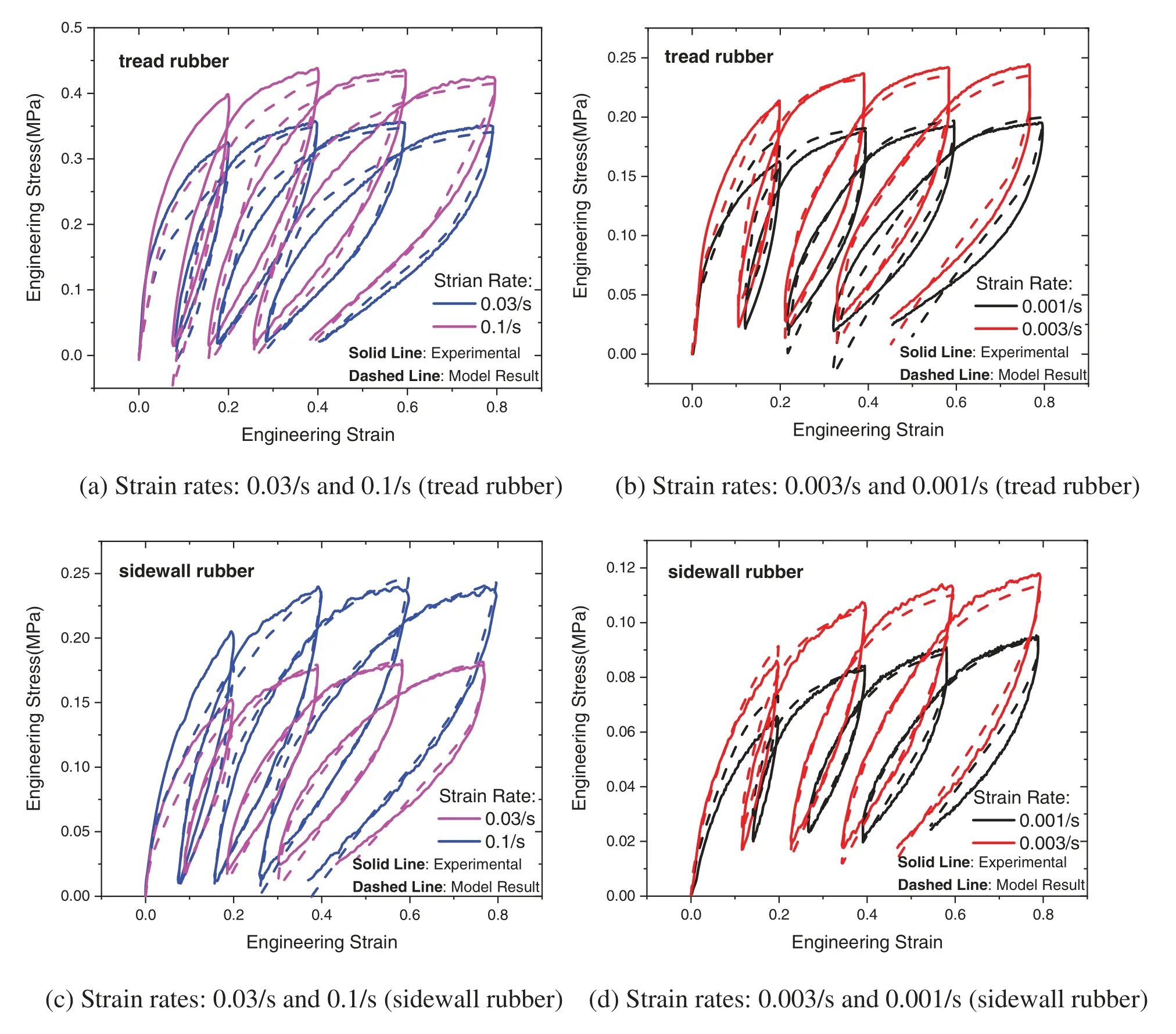
Figure 5:The fitting results using the parallel network model

Table 1: The ultimate optimization parameters for the tread rubber

3 Finite Element Simulation of the Radial Tire Building Process

During the tire building process,the tread pattern has not been formed and all the components are distributed axisymmetrically with respect to the axial of the building drums.Hence,the simulation is carried out in a two-dimensional (2D) axisymmetric setting that only takes into account circumferential tread grooves.The tire components are also bilaterally symmetric,and only half of the axisymmetric model is required for simulation.Consequently,the number of degrees of freedom of the finite element model is greatly decreased,and the simulation can be completed faster in comparison to a full three-dimensional model.The tire building process is always carried out at room temperature,so the temperature effect is not considered during simulation.

The finite element software ABAQUS[46]was used for the simulation process.Considering the incompressibility of the uncured rubber,the element type used is a hybrid large deformation solid element,and the cord reinforcements embedded in rubber components are simulated using the socalled rebar element,which is a kind of one-dimensional(1D)bar element.The constitutive model of the steel is used for the rebar element.To improve the calculation accuracy,relatively small mesh sizes are used(1.0 to 1.5 mm),and the model is meshed into 8892 elements.

According to the process sequence,the overall tire building operations can be divided into four steps: component winding process,rubber bladder inflation,component stitching and carcass band folding-back.

3.1 Component Winding Process on Building Drums

The component winding process includes the components winding on the main drum and auxiliary drum.The components wound on the main drum include sidewall,innerliner,carcass,shoulder,bead flipper,bead and so on,and the components wound on the auxiliary drum include belts,tread and some rubber sheets.

In production,the component plies(sidewall first)are wound around the building drum layer by layer.Fig.6 illustrates the simulation of the sidewall winding process on the main drum.The length of the component is less than the circumference of the drum.Therefore,the displacement boundary condition is first applied to the inner surface to stretch the component circumferentially,as shown in Fig.6a.Then,the contact pair between the component and the drum is activated,and the displacement constraint is released to make the component adhere to the cylindrical forming drum(Figs.6b and 6c).Subsequently,the second component can be fitted on the upper surface of the previous component in the same way.After the carcass is wound on the main drum,a uniformly distributed pressure is applied on the upper surface of the carcass in the simulation to model the pressing of the pressure-roller to bond different components together tightly and simultaneously to squeeze the air that might be entrapped between the plies out (Fig.7a).Thus,all the components on the main drum are assembled into a“carcass band”.After that,two beads are installed surrounding the drum to be positioned immediately above the bead locking apparatus,as shown in Fig.7b.Finally,the bead locking apparatus radially expends to push the material outward to clamp the bead over the circumference of the building drum,as depicted in Fig.7c.The beads that are “locked”by the locking segments can keep the tire firmly seated on the main drum during the subsequent building process.It should be noted that in the current and subsequent building or shaping processes,there are two kinds of contact conditions:the contact between building drums and rubber components and the contact between two rubber components.The uncured rubber is very sticky,so the contact between two rubber components cannot be separated once established,while the contact between rubber components and building drums is free to separate during the building process.The friction coefficient between the two rubber components is taken as 1.2,and the friction coefficient between the rubber components and building drums is taken as 0.5.

Figure 6: Component winding process on the main drums (a) Applying displacement boundary conditions(b)Releasing displacement boundary conditions(c)Completing the winding process

The component winding processes on the auxiliary drum are carried out in the same way.The belt/tread band is established by sequentially bonding components including different belts and the tread rubber on the auxiliary drum.After the tread is assembled,a uniformly distributed pressure is applied on the upper surface of the tread by a pressure-roller to bond different parts together tightly,as shown in Fig.8b.

Figure 7:Component winding process on the main drums(a)Pressing components together using a pressure-roller (b) Each of the beads is moved to surround the drum (c) The bead locking segment expands radially to clamp the bead

Figure 8: Component winding process on the auxiliary drums (a) Initial position of the different components on the auxiliary drum(b)Pressing components together using a pressure-roller

3.2 Building Process of the Green Tire

The following building process of the green tire is performed in three stages: rubber bladder inflation,component stitching and carcass band folding-back.Fig.9 depicts the whole shaping process.

Figure 9:Building process of the green tire(a)Move belt/tread band to the main drum(b)Inflate the rubber bladder(c)Assemble the belt/tread band onto carcass band(d)Component stitching(e)Fold the carcass band back(f)The final green tire

After the winding process of different components on the main drum and the auxiliary drum,the belt/tread band is first detached from the auxiliary drum,which was gripped from the outside circumferentially,and then is moved to the central section of the main drum to surround the carcass band (Fig.9a).In the central section of the building drum,there is a rubber bladder that was subsequently inflated,whereby the components between two sets of beads are radially expanded and shaped to a toroidal form.Here,in the simulation model,uniformly distributed inflation pressure is directly applied on the inner surface of the green tire to simplify the analysis,as shown in Fig.9b,in which the center portion of the toroidally bulged carcass band is supported by inflation pressure(Pressure 1).During inflation,both sides of the carcass band are displaced close to each other integrally with the bead locking apparatus.Eventually,the belt/tread band is assembled onto the radially expanded carcass band,as shown in Fig.9c,where contact is established between the belts and the carcass band.What follows is the component stitching process in Fig.9d.To stitch different rubber components tightly,the distributed pressures are applied on the upper surface of the tread and the bead filler by several pressing rollers,with the inflation pressure(Pressure 1)inside the rubber bladder and the bead locking apparatus fixed.Next,the two end portions of the carcass band are folded back tightly along the outer contour of the toroidally bulged carcass band to complete the assembly of all components,as shown in Fig.9e,where the folding-back roller is modeled using an analytical rigid body and the roller speed remains consistent with the practical pressing process.Finally,all the boundary conditions are removed,and the green tire building process is completely simulated(Fig.9f).From the figure,it can be observed that there are holes between uncured rubber layers in the final simulated green tire.This means that a small amount of air is still entrapped between component plies.This is consistent with the past section cutting experiments of the green tire.Without considering the convergence problems,the computational time for the whole tire building process is about 13 h(Intel(R)Xeon(R)CPU E5-2678,12 threads).

4 Finite Element Simulation of the Radial Tire Shaping Process

In the actual tire shaping process,the green tire is first placed inside a large mold.Then,the inner pressure is applied inside the bladder to give the green tire its final shape,and heat energy is simultaneously applied to stimulate the chemical reaction between the rubber and other materials.In this study,the focus is on the deformation of the tire in the early shaping stage.The chemical reaction is not considered,and the physical property changes of rubber materials are neglected due to the small temperature change and very low SOC in this stage.

In the tire shaping simulation,the contact conditions are consistent with the previous building process.The whole tire shaping process is depicted in Fig.10.First,the rubber bladder was evacuated,and the green tire was placed inside the opened mold.Second,a low inner pressure is applied to the rubber bladder to establish contact between the bladder and the green tire(Fig.10b).Due to the low stiffness of the green tire,the tire is expanded,and the beads are pressed to the two sides of the mold.The green tire is now only held by contact with the bladder and mold.Next,the upper side of the mold moves down,Fig.10c,and the middle of the mold is subsequently closed up to its final position,Fig.10d,still with the low inner pressure.Finally,the inner pressure is increased to a higher value to press the green tire to its final position(Figs.10e and 10f).During this step,the tire will change its shape significantly,where the viscoelasticity of the uncured rubber relaxes and the material flows further into the edges of the mold to form circumferential grooves.Fig.10f shows that the pattern grooves on the mold are completely filled except for the two small corners in the middle groove,where further rubber flow may require the promoting effect of temperature.Note that the holes between the uncured rubber layers in the simulated green tire completely disappeared during the shaping process,which means that the entrapped air could be expelled thoroughly in this process.And the computational time for the whole tire shaping process is about 4.8 h.

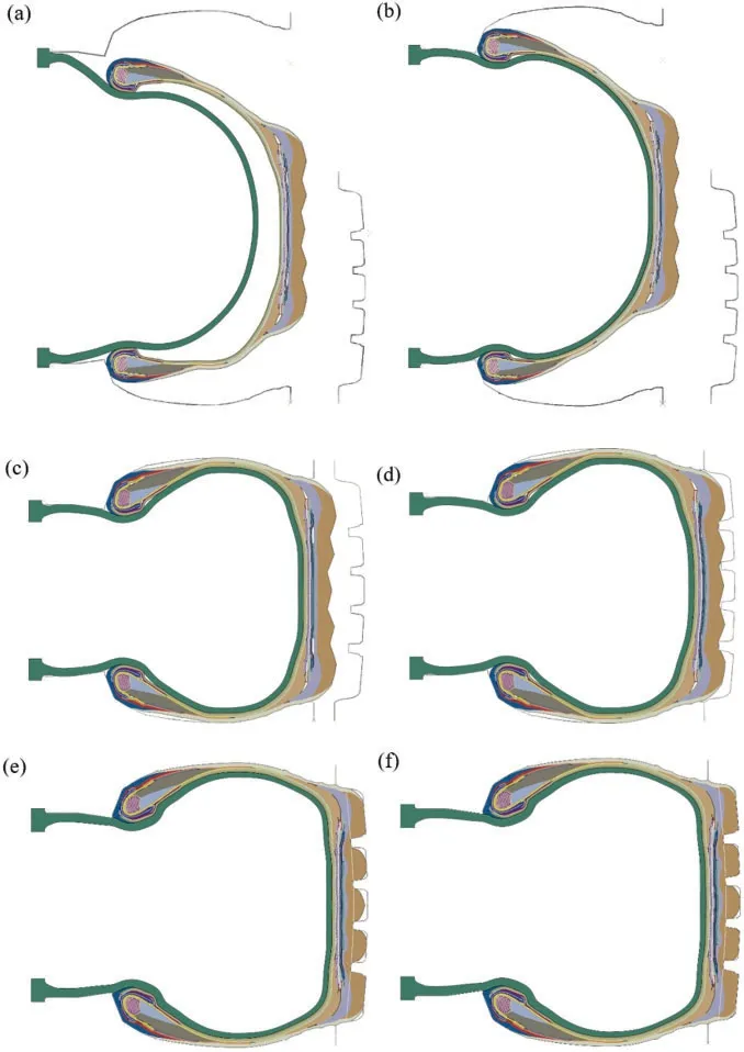
Figure 10:Tire shaping process(a)Place green tire inside the mold(b)Inflate the rubber bladder(c)Upper mold moves down (d) Move middle mold in position (e) Increase the inner pressure (f) The final shaped radial tire

5 Finite Element Simulation Results and Discussion

5.1 Experimental Verification of the Tire Building Simulation

To verify the validity of the simulation method,the contour of the profile obtained by simulation of the tire building process is accordingly compared with experimentation.The experimentation of the section contour was obtained by 3D scanning through the 3D hand-held scanner.Due to symmetry,only half of the profile is analyzed.

Fig.11 shows the comparison between the numerical prediction of the green tire profile and the experimental profile.For convenience,the axes of symmetry of the two profiles remain aligned.It can be observed that the contours of the cross-section calculated by the simulation are basically consistent with the experimental observations.Notably,the 3D scanning process usually takes some time,and the green rubber continues to deform during the scanning process,which eventually leads to some difference between the two profiles,that is,the deviation between the two contours in the bead section,as shown in Fig.11.Hence,to eliminate the influence of the green tire deformation and ensure a more accurate comparison,the section thicknesses at different positions for both green tire profiles were measured,and the comparison results are given in Table 2.It can be seen from the table that the section thicknesses of the simulation result of the green tire are in good agreement with the 3D scanning result of the produced green tire.

Figure 11:Comparison of the contours of the profiles between the simulation and experimentation

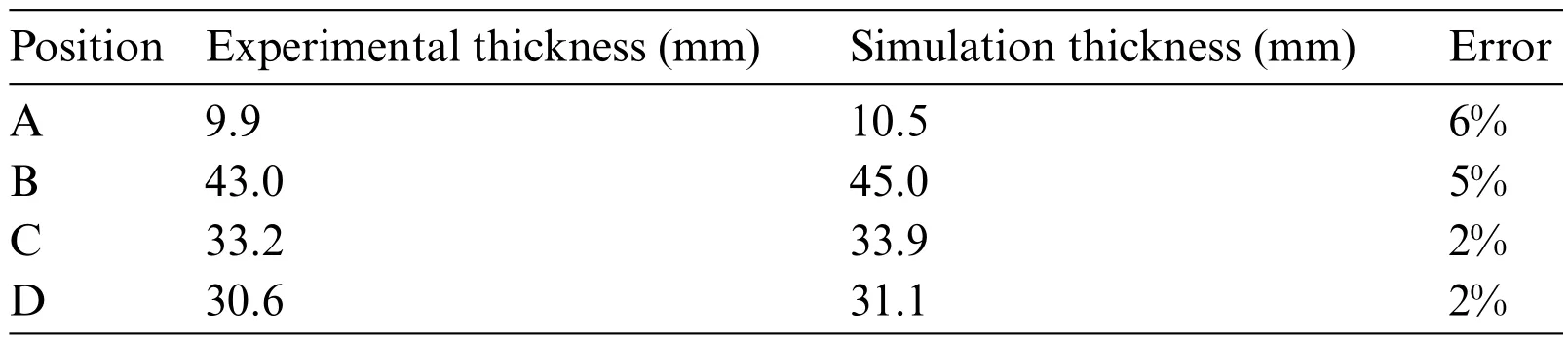
Table 2: The section thicknesses at different positions

The profile of the tire after the shaping process was not compared with experimentation because for both cases the outer contour is exactly the same as the inner contour of the mold.

5.2 Production Defect Optimization

Tire manufacturing,which includes the building process and shaping process,is such a complex process that some product defects inevitably appear in production [47].Due to the complex process parameters,the causes of these product defects are very difficult to determine,even for experienced engineers.Through finite element simulation,the influence of process parameters on the final products can be observed intuitively,thereby helping engineers adjust production parameters to eliminate product defects.

In this section,the effect of the parameter“drum width”is investigated.During the component winding process,the distance between the inner sides of two beads on the building drum is usually called the drum width.As discussed above,the beads that are “locked”by the locking segments in the component winding process can prevent the plies of rubber components from sliding inward or outward during the subsequent building process.Consequently,the length of the drum width directly affects the final tire structure.If the drum width is too long or too short,defects come into being.Fig.12 shows the simulation result of the shaping process when the drum width increases by 10 mm.It can be observed that the increasing drum width causes obvious“shoulder flection”,where both cord and rubber components bend considerably.In contrast,when the drum width decreases,“shoulder flection”does not occur,but the force on the carcass cord increases sharply,which may lead to other production defects(Fig.13).

Figure 12:The simulation result of the shaping process with drum width increasing 10 mm(a)After the mold is closed(b)After the inner pressure increases

Figure 13: The simulation result of the shaping process with drum width decreasing 10 mm (a) The final tire shape(b)The change of cord force

To verify the simulation results,an experiment was carried out to produce a tire with the drum width increased by 10 mm.The X-ray images of the tire shoulder are presented in Fig.14.From the figure,it can be seen that carcass cord distortion clearly occurred in the shoulder after the drum width increased.Hence,moderately reducing the drum width can be adopted to eliminate the shoulder flection defect in tire production.

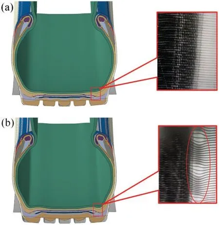
Figure 14: X-ray images of the tire shoulder (a) tire with reasonable production parameters (b) tire with the drum width increased by 10 mm

Therefore,the simulation strategy,which includes the whole tire production process from semifinished parts to the final finished tire,can be quite helpful to observe the influence of parameter changes.Thus,parameter investigations can be performed to improve the production process and eliminate product defects conveniently.

6 Conclusions

In the present study,the tensile mechanical properties of uncured rubber from different components were first investigated at different strain rates.Experimental investigations show that the tensile mechanical responses of the uncured rubber are highly rate-dependent and that the different uncured rubber compounds have similar mechanical characteristics,including a distinct hysteresis effect,residual strain and rate dependence.To describe the constitutive behaviors of the uncured rubber,an elasto-viscoplastic constitutive model based on the eight-chain model and Bergstrom-Boyce flow was adopted.This model characterizes the nonlinear mechanical behaviors of uncured rubber well.

The finite element models of each component of a radial tire were established,and the whole tire building process(including the component winding process,rubber bladder inflation,component stitching and carcass band folding-back) and the shaping process were simulated using the elastoviscoplastic constitutive model.From the simulation,the entrapped air between component plies can be observed during the tire building process.The tire shaping process can help to expel the entrapped air.The simulated green tire profile was compared with the actual profile obtained through 3D scanning,and the two overlapped well,which verified the reliability of the simulation process.The deformation and stress distribution of the rubber components and cord plies can all be obtained through the simulation.Therefore,the simulation method can be used to judge the rationality of the tire construction design and provide guidance for the real tire manufacturing process.

The effect of the parameter “drum width” was investigated using the simulation method.An unreasonable drum width can lead to obvious production defects.If the drum width is too long,the“shoulder flection”usually occurs.In contrast,if the drum width is too short,the force on the carcass cord can increase sharply,which may result in other production defects.An experiment with drum width increased by 10 mm was carried out,and the carcass cord arrangement after the shaping process was observed through X-ray.The experimental results verified the prediction of the simulation.

Authors’Contribution:All authors have an equivalent contribution.

Acknowledgement: The support of the long-term technological cooperation project between Giti Tire Company and USTC is gratefully acknowledged.

Funding Statement:This work was funded by the National Natural Science Foundation of China(Nos.11902229,11502181)and the Strategic Priority Research Program of the Chinese Academy of Sciences(Grant Nos.XDB22040502,XDC06030200).

Conflicts of Interest:The authors declare that they have no conflicts of interest to report regarding the present study.

Appendix A

The invariants of the right Cauchy-Green tensor C are:

The Cauchy stressσis obtained by proper differentiation of the strain energy density with respect to the corresponding deformations:

Inserting the invariants into Eq.(A.4)gives the following expression for the Cauchy stress:

For rubber-like incompressible materials,the equation can be simplified to:

For the eight-chain model,the strain energy density,U,can be written as:

wherenis the average chain density (number of molecular chains per unit reference volume),Nis the average number of“rigid links”between two molecular joints,β=Lis the Langevin function defined asL(x)=cothx−1/x,λchain=is the effective chain stretch in whichI1is the first invariant of the right Cauchy-Green tensor,kBis Boltzmann’s constant,andΘis the reference temperature.

Substituting Eq.(A.7)into Eq.(A.6)and applying the chain rules of differentiation,the relaxed Cauchy stress is written as follows[31]:

The shear modulus can be defined as:

Hence,the Cauchy stress can be written as: