Bayesian Computation for the Parameters of a Zero-Inflated Cosine Geometric Distribution with Application to COVID-19 Pandemic Data

Sunisa Junnumtuam,Sa-Aat Niwitpongand Suparat Niwitpong

Department of Applied Statistics,Faculty of Applied Science,King Mongkut’s University of Technology North Bangkok,Bangkok,10800,Thailand

ABSTRACT A new three-parameter discrete distribution called the zero-inflated cosine geometric (ZICG) distribution is proposed for the first time herein.It can be used to analyze over-dispersed count data with excess zeros.The basic statistical properties of the new distribution,such as the moment generating function,mean,and variance are presented.Furthermore,confidence intervals are constructed by using the Wald,Bayesian,and highest posterior density (HPD) methods to estimate the true confidence intervals for the parameters of the ZICG distribution.Their efficacies were investigated by using both simulation and real-world data comprising the number of daily COVID-19 positive cases at the Olympic Games in Tokyo 2020.The results show that the HPD interval performed better than the other methods in terms of coverage probability and average length in most cases studied.

KEYWORDS Bayesian analysis;confidence interval;gibbs sampling;random-walk metropolis;zero-inflated count data

1 I ntroduction

Over-dispersed count data with excess zeros occur in various situations,such as the number of torrential rainfall incidences at the Daegu and the Busan rain gauge stations in South Korea [1],the DMFT (decayed,missing,and filled teeth) index in dentistry [2],and the number of falls in a study on Parkinson’s disease[3].Classical models such as Poisson,geometric,and negative binomial(NB) distributions may not be suitable for analyzing these data,so two classes of modified count models(zero-inflated(ZI)and hurdle)are used instead.Both can be viewed as finite mixture models comprising two components:for the zero part,a degenerate probability mass function is used in both,while for the non-zero part,a zero-truncated probability mass function is used in hurdle models and an untruncated probability mass function is used in ZI models.Poisson and geometric hurdle models were proposed and used by [4] to analyze data on the daily consumption of various beverages; in the intercept-only case(no regressors appear in either part of the model),the ZI model is equivalent to the hurdle model,with the estimation yielding the same log-likelihood and fitted probabilities.Furthermore,several comparisons with classical models have been reported in the literature.The efficacies of ZI and hurdle models have been explored by comparing least-squares regression with transformed outcomes(LST),Poisson regression,NB regression,ZI Poisson(ZIP),ZINB,zero-altered Poisson (ZAP) (or Poisson hurdle),and zero-altered NB (ZANB) (or NB hurdle) models [5]; the results from using both simulated and real data on health surveys show that the ZANB and ZINB models performed better than the others when the data had excess zeros and were over-dispersed.Recently,Feng[6]reviewed ZI and hurdle models and highlighted their differences in terms of their data-generating process;they conducted simulation studies to evaluate the performances of both types of models,which were found to be dependent on the percentage of zero-deflated data points in the data and discrepancies between structural and sampling zeros in the data-generating process.

The main idea of a ZI model is to add a proportion of zeros to the baseline distribution [7,8],for which various classical count models (e.g.,ZIP,ZINB,and ZI geometric (ZIG)),are available.These have been studied in several fields and many statistical tools have been used to analyze them.The ZIP distribution originally proposed by[9]has been studied by various researchers.For instance,Ridout et al.[10]considered the number of roots produced by 270 shoots ofTrajanapple cultivars(the number of shoots entries provided excess zeros in the data),and analyzed the data by using Poisson,NB,ZIP,and ZINB models;the fits of these models were compared by using the Akaike information criterion (AIC) and the Bayesian information criterion (BIC),the results of which show that ZINB performed well.Yusuf et al.[11]applied the ZIP and ZINB regression models to data on the number of falls by elderly individuals;the results show that the ZINB model attained the best fit and was the best model for predicting the number of falls due to the presence of excess zeros and over-dispersion in the data.Iwunor[12]studied the number of male rural migrants from households by using an inflated geometric distribution and estimated the parameters of the latter;the results show that the maximum likelihood estimates were not too different from the method of moments values.Kusuma et al.[13]showed that a ZIP regression model is more suitable than an ordinary Poisson regression model for modeling the frequency of health insurance claims.

The cosine geometric (CG) distribution,a newly reported two-parameter discrete distribution belonging to the family of weighted geometric distributions[14],is useful for analyzing over-dispersed data and has outperformed some well-known models such as Poisson,geometric,NB,and weighted NB.In the present study,the CG distribution was applied as the baseline and then a proportion of zeros was added to it,resulting in a novel three-parameter discrete distribution called the ZICG distribution.

Statistical tools such as confidence intervals provide more information than point estimation andp-values for statistical inference [15].Hence,they have often been applied to analyze ZI count data.For example,Wald confidence intervals for the parameters in the Bernoulli component of ZIP and ZAP models were constructed by[16],while Waguespack et al.[17]provided a Wald-based confidence interval for the ZIP mean.Moreover,Srisuradetchai et al.[18]proposed the profile-likelihood-based confidence interval for the geometric parameter of a ZIG distribution.Junnumtuam et al.[19]constructed Wald confidence intervals for the parameters of a ZIP model;in an analysis of the number of daily COVID-19 deaths in Thailand using six models: Poisson,NB,geometric,Gaussian,ZIP,and ZINB,they found that the Wald confidence intervals for the ZIP model were the most suitable.Furthermore,Srisuradetchai et al.[20]proposed three confidence intervals:a Wald confidence interval and score confidence intervals using the profile and the expected or observed Fisher information for the Poisson parameter in a ZIP distribution;the latter two outperformed the Wald confidence interval in terms of coverage probability,average length,and the coverage per unit length.

Besides the principal method involving maximum likelihood estimation widely used to estimate parameters in ZI count models,Bayesian analysis is also popular.For example,Cancho et al.[21]provided a Bayesian analysis for the ZI hyper-Poisson model by using the Markov chain Monte Carlo(MCMC) method; they used some noninformative priors in the Bayesian procedure and compared the Bayesian estimators with maximum likelihood estimates obtained by using the Newton-Raphson method and found that all of the estimates were close to the real values of the parameters as the sample size was increased,which means that their biases and mean-squared errors(MSEs)approached zero under this circumstance.Recently,Workie et al.[22]applied the Bayesian analytic approach by using MCMC simulation and Gibbs’sampling algorithm for modeling the Bayesian ZI regression model determinants to analyze under-five child mortality.

Motivated by these previous studies,we herein propose Wald confidence intervals based on maximum likelihood estimation,Bayesian credible intervals,and highest posterior density (HPD)intervals for the three parameters of a ZICG distribution.Both simulated data and real-world data were used to compare the efficacies of the proposed methods for constructing confidence intervals via their coverage probabilities and average lengths.

2 Methodology

2.1 The ZICG Distribution

The CG distribution is a two-parameter discrete distribution belonging to the family of weighted geometric distributions[14].The probability mass function(PMF)for a CG distribution is given by

whereθ∈and

Ifθ=0,then we can obtainCp,θ=1−pandYis a standard geometric distribution.LetXbe a random variable following a ZICG distribution with parametersω∈(0,1),p∈(0,1),andθ∈Subsequently,we can construct a new three-parameter discrete distribution with CG as the baseline distribution,and so the pmf ofXis given by

whereωis the probability of zeros and 0≤ω≤1.Moreover,one can easily prove(X=x)=1.Fig.1 provides pmf plots for the ZICG distribution for different parameter combinations.It can be seen that even though the proportion of zeros (ω) is small (i.e.,ω=0.1),the probability of zeros is still high;e.g.,ω=0.1,p=0.5,andθ=1 providesP(X=0) >0.5.Moreover,whenpis large,the dispersion is high.Overall,the ZICG distribution,which is suitable for data that are over-dispersed with excess zeros,can be used to analyze ZI count data.

2.2 Statistical Properties

This section provides the cumulative distribution function (CDF),moment generating function(MGF),mean,and variance of a ZICG distribution,which are derived from the CG distribution[14].

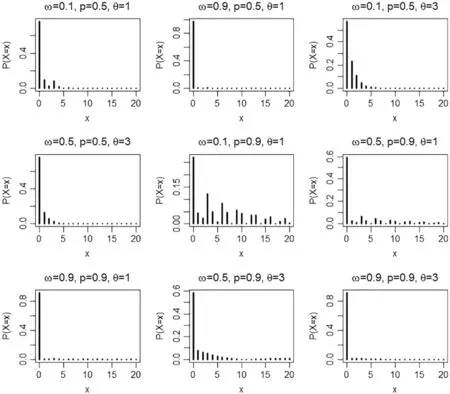
Figure 1:Pmf plots of the ZICG distribution for different values of the parameters ω,p,and θ

Proposition 2.1.The cdf of a ZICG distribution with parametersω,p,andθis given by

Proposition 2.2.The mgf of the ZICG distribution with parametersω,p,andθis given by

Since the explicit expression for the moment using equality isμ′r=E(Xr)=M(r)(t) |t=0,then the first two moments respectively become

SinceM′X(t=0)=E(X),then

andMX′′(t=0)=E(X2),then

SinceV(X)=E(X2)−(E(X))2,then

The index of dispersion(D),a measure of dispersion,is defined as the ratio of the variance to the mean

The values ofDfor selected values of the parametersω,p,andθare provided in Table 1.When the value of parameterpincreases,the index of dispersion also increases,and so the value ofpaffectsDmuch more than parametersωandθ.

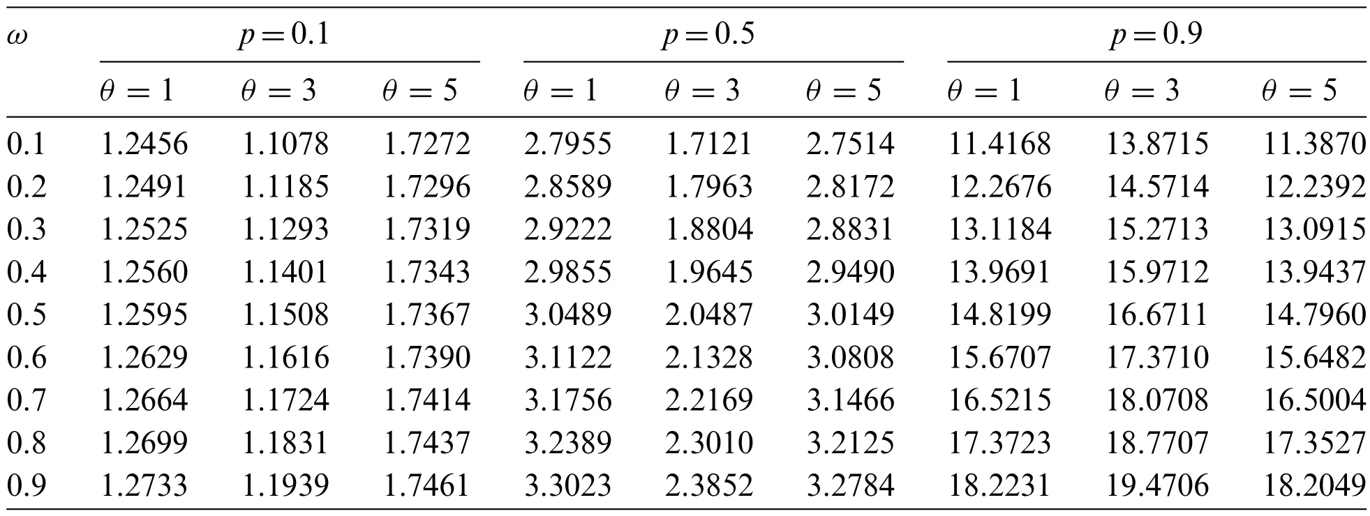
Table 1: Index of dispersion of the ZICG distribution for different values of parameters

2.3 Maximum Likelihood Estimation for the ZICG Model with No Covariates

The likelihood function of the ZICG distribution is

while the log-likelihood function of the ZICG distribution can be expressed as

In the case of a single homogeneous sample(p,θ,andωare constant or have no covariates),the log-likelihood function can be written as

whereJis the largest observed count value;njis the frequency of each possible count value;j=x=0,1,2,...,J;n0is the number of observed zeros;and=nis the total number of observations or the sample size.Based on log-likelihood function(13),maximum likelihood estimates ˆω,ˆp,and ˆΘare the roots of equationsandrespectively.

Here,we have

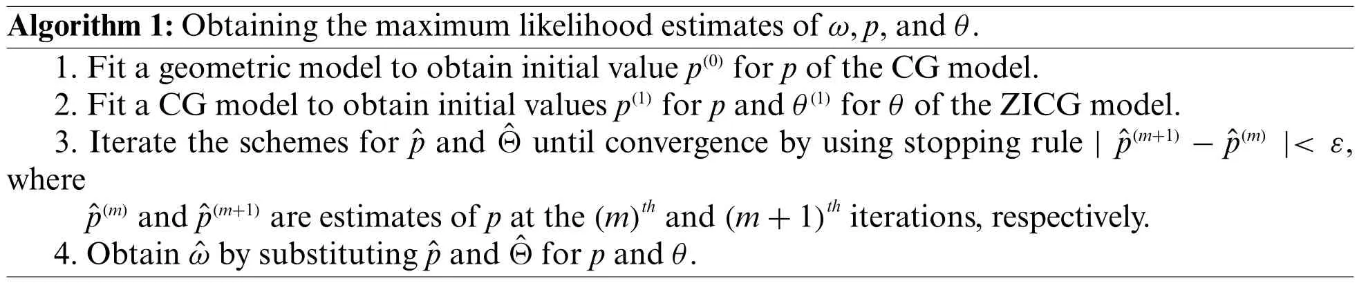
Algorithm 1:Obtaining the maximum likelihood estimates of ω,p,and θ.1.Fit a geometric model to obtain initial value p(0)for p of the CG model.2.Fit a CG model to obtain initial values p(1)for p and θ(1)for θ of the ZICG model.3.Iterate the schemes for ˆp and ˆΘ until convergence by using stopping rule | ˆp(m+1)−ˆp(m) |< ε,where ˆp(m)and ˆp(m+1)are estimates of p at the(m)th and(m+1)th iterations,respectively.4.Obtain ˆω by substituting ˆp and ˆΘ for p and θ.

This provides the closed-form expression for,and so iteration is not required.However,since there are no closed-form expressions forand,they are solved by using an educated version of trialand-error.The general idea is to start with an initial educated guess of the parameter value,calculate the log-likelihood for that value,and then iteratively find parameter values with larger and larger log-likelihoods until no further improvement can be achieved.There are a variety of fast and reliable computational algorithms for carrying out these procedures,one of the most widely implemented being the Newton-Raphson algorithm[23].In this study,the maximum likelihood estimates of,,andcan be obtained by solving the resulting equations simultaneously by using thenlmfunction in[24].

2.4 The Wald Confidence Intervals for the ZICG Parameters

In this study,we assume that there is more than one unknown parameter.Meanwhile,the assumed parameter vector is=(β1,...,βk)Tand the maximum likelihood estimator for it is;i=1,2,...,k,wherekis the number of parameters.Thus,

where

Hence,the(1−α)100%Wald confidence interval can be constructed as

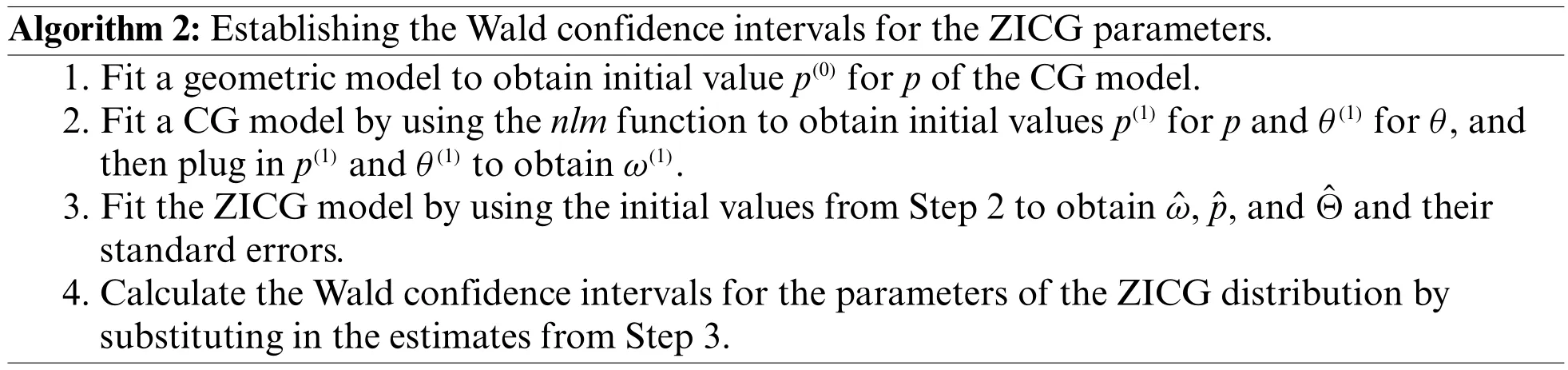
Algorithm 2:Establishing the Wald confidence intervals for the ZICG parameters.1.Fit a geometric model to obtain initial value p(0)for p of the CG model.2.Fit a CG model by using the nlm function to obtain initial values p(1)for p and θ(1)for θ,and then plug in p(1)and θ(1)to obtain ω(1).3.Fit the ZICG model by using the initial values from Step 2 to obtain ˆω,ˆp,and ˆΘ and their standard errors.4.Calculate the Wald confidence intervals for the parameters of the ZICG distribution by substituting in the estimates from Step 3.

2.5 Bayesian Analysis for the Confidence Intervals for the ZICG Parameters

SupposeX=x1,x2,...,xnis a sample from ZICG(ω,p,θ),then the likelihood function for the observed data is given by

LetA=xi:xi=0,i=1,...,nandmbe the numbers in setA,then the likelihood function for ZICG can be written as

Since the elements in setAcan be generated from two different parts:(1)the real zeros part and(2)the CG distribution,after which the an unobserved latent allocation variable can be defined as

wherei=1,...,mand

Thus,the likelihood function based on augmented dataD={X,I},whereI=(I1,...,Im) [25]becomes

whereS=∼Bin[m,p(ω,p,θ)].Thus,the likelihood function for ZICG based on the augmented data becomes

and

Since there is no prior information from historic data or previous experiments,we use the noninformative prior for all of the parameters.The prior distributions forωandpare assumed to be beta distributions while that ofθis assumed to be a gamma distribution.Thus,the joint prior distribution for ZICG is

whereB(a,b)=andB(c,d)=In this study all of the parameters are assumed to have prior specifications,which areω∼Beta(1.5,1.5),p∼Beta(2,5),andθ∼Gamma(2,1/3).Since the posterior distributions for the parameters can be formed as[7]

the joint posterior distribution for parametersω,p,andθcan be written as

Since the joint posterior distribution in (35) is analytically intractable for calculating the Bayes estimates similarly to using the posterior distribution method,MCMC simulation can be applied to generate the parameters [26,27].The Metropolis-Hastings algorithm is an MCMC method for obtaining a sequence of random samples from a probability distribution from which direct sampling is difficult.Subsequently,the obtained sequence can be used to approximate the desired distribution.Moreover,the Gibbs’sampler,which is an alternative to the Metropolis-Hastings algorithm for sampling from the posterior distribution of the model parameters,can be used.Hence,the Gibbs’sampler can be applied to generate samples from the joint posterior distribution in(35).Clearly,the marginal posterior distribution ofωgivenpandθis

Thus,the marginal posterior distribution ofωisBeta(S+a,n−S+b),and the marginal posterior distribution ofpgivenωandθis

and the marginal posterior distribution ofθgivenωandpis

Here,we applied the random-walk Metropolis (RWM) algorithm to generatepandθ.RWM is defined by using transition probabilityp(x→y) for one valuextoyso that the distribution of points converges toπ(x).Since RWM is a special case of the Metropolis-Hastings algorithm withp(x,y)=p(y,x)(symmetric)[28],then the acceptance probability can be calculated as

The process proceeds as follows:

1.Choose trial positionYj=Xj−1+∊j,where∊jis a random perturbation with distributiongthat is symmetric(e.g.,a normal distribution).

2.Calculater=

3.GenerateUjfromUniform[0,1].

4.IfUj≤α(Xj−1,Yj),then accept the change and letXj=Yj,else letXj=Xj−1.

The Gibbs’sampling steps are as follows:

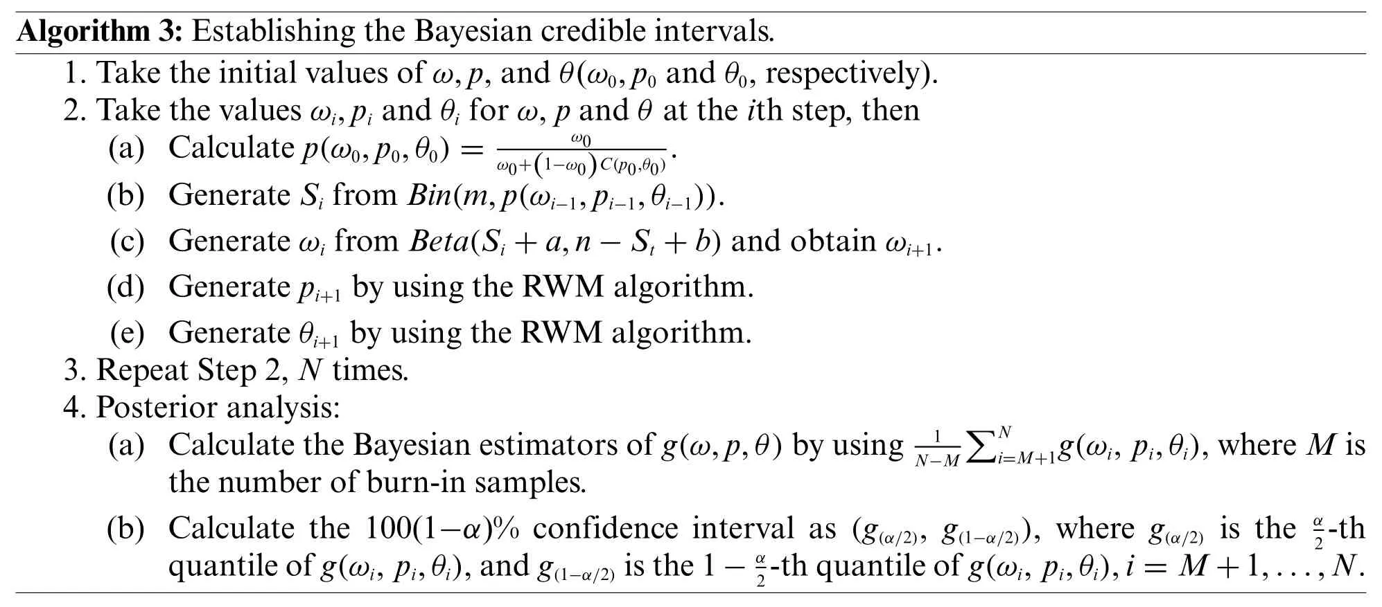
Algorithm 3:Establishing the Bayesian credible intervals.1.Take the initial values of ω,p,and θ(ω0,p0 and θ0,respectively).2.Take the values ωi,pi and θi for ω,p and θ at the ith step,then(a) Calculate p(ω0,p0,θ0)=ω0 ω0+(1−ω0)C(p0,θ0).(b) Generate Si from Bin(m,p(ωi−1,pi−1,θi−1)).(c) Generate ωi from Beta(Si+a,n−St+b)and obtain ωi+1.(d) Generate pi+1 by using the RWM algorithm.(e) Generate θi+1 by using the RWM algorithm.3.Repeat Step 2,N times.4.Posterior analysis:(a) Calculate the Bayesian estimators of g(ω,p,θ)by using1ΣNi=M+1g(ωi,pi,θi),where M is the number of burn-in samples.(b) Calculate the 100(1−α)% confidence interval as (g(α/2),g(1−α/2)),where g(α/2) is the α N−M 2-th quantile of g(ωi,pi,θi),and g(1−α/2)is the 1−α 2-th quantile of g(ωi,pi,θi),i=M+1,...,N.

2.6 The Bayesian-Based HPD Interval

The HPD interval is the shortest Bayesian credible interval containing 100(1−α)% of the posterior probability such that the density within the interval has a higher probability than outside of it.The two main properties of the HPD interval are as follows[29]:

1.The density for each point inside the interval is greater than that for each point outside of it.

2.For a given probability(say 1−α),the HPD interval has the shortest length.

Bayesian credible intervals can be obtained by using the MCMC method[30].Hence,we used it to construct HPD intervals for the parameters of a ZICG distribution.This approach only requires MCMC samples generated from the marginal posterior distributions of the three parameters:ω,p,andθ.In the simulation and computation,the HPD intervals were computed by using theHDIntervalpackage version 0.2.2[31]from the R statistics program.

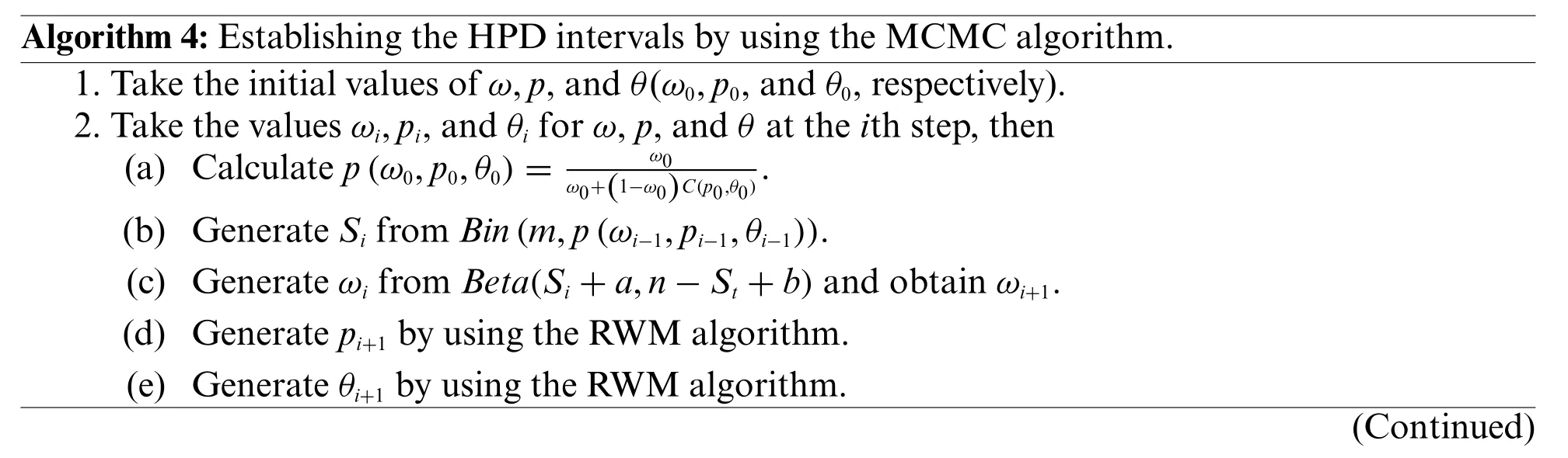
Algorithm 4:Establishing the HPD intervals by using the MCMC algorithm.1.Take the initial values of ω,p,and θ(ω0,p0,and θ0,respectively).2.Take the values ωi,pi,and θi for ω,p,and θ at the ith step,then(a) Calculate p(ω0,p0,θ0)=ω0 ω0+(1−ω0)C(p0,θ0).(b) Generate Si from Bin(m,p(ωi−1,pi−1,θi−1)).(c) Generate ωi from Beta(Si+a,n−St+b)and obtain ωi+1.(d) Generate pi+1 by using the RWM algorithm.(e) Generate θi+1 by using the RWM algorithm.(Continued)

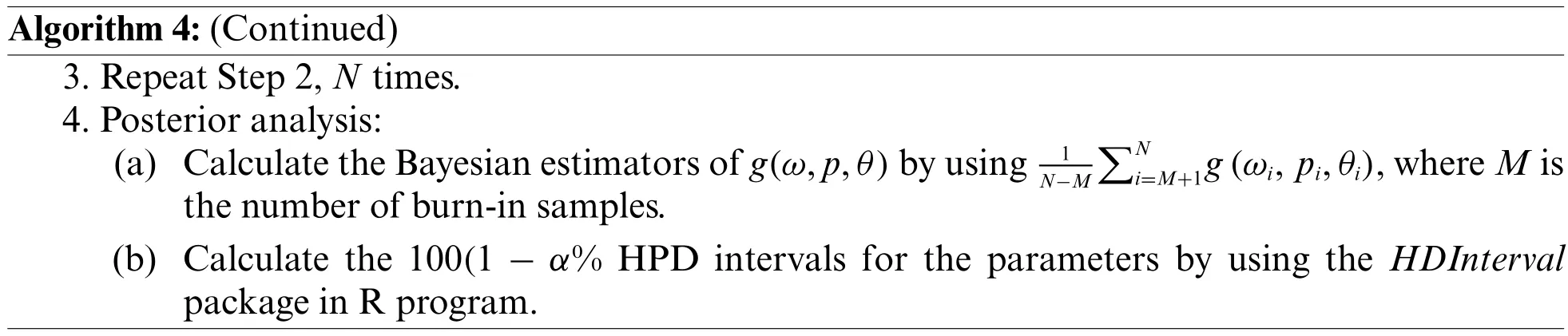
Algorithm 4:(Continued)3.Repeat Step 2,N times.4.Posterior analysis:(a) Calculate the Bayesian estimators of g(ω,p,θ)by using1ΣNi=M+1g(ωi,pi,θi),where M is the number of burn-in samples.(b) Calculate the 100(1−α% HPD intervals for the parameters by using the HDInterval package in R program.N−M

2.7 The Efficacy Comparison Criteria

Coverage probabilities and average lengths were used to compare the efficacies of the confidence intervals.Suppose the nominal confidence level is 1−α,then confidence intervals that provide coverage probabilities of 1−αor better are selected.In addition,the shortest average length identifies the best confidence interval under the provided conditions.LetC(s)=1 if the parameter values fall within the confidence interval range,elseC(s)=0.The coverage probability is computed by

and the average length is computed by

whereU(s)andL(s)are the upper and lower bounds of the confidence interval for loops,respectively.

3 Results and Discussion

3.1 Simulation Study

Sample sizen=50 or 100; proportion of zerosω=0.1,0.5,or 0.9;p=0.5 or 0.9; andθ=1 or 3 were the parameter values used in the simulation study.The simulation data were generated by using the inverse transform method[32],with the number of replications set as 1,000 and the nominal confidence level as 0.95.A flowchart of the simulation study is presented in Fig.2,while the coverage probabilities and average lengths of the methods are reported in Table 2.

For sample sizen=50 or 100,the Bayesian credible intervals and the HPD intervals performed better than the Wald confidence intervals because they provided coverage probabilities close to the nominal confidence level(0.95)and obtained the shorter average lengths for almost all of the cases.However,when the proportion of zeros was high(i.e.,ω=0.9),none of the methods performed well.In addition,the average lengths of all of the methods decreased forn=100 compared ton=50.Overall,the Wald confidence intervals did not perform well,which might have been caused by poor optimization that can sometimes occur.Thus,the optimization was not a good choice in this case.Similarly,Srisuradetchai et al.[20] found that when the Poisson parameter has a low value and the sample size is small,the Wald confidence interval for the Poisson parameter of a ZIP distribution was inferior to the other two intervals tested.Moreover,for a small sample size,the coverage probabilities of the Wald confidence intervals tended to decrease as the proportion of zeros was increased.Likewise,Daidoji et al.[33]showed that the Wald-type confidence interval for the Poisson parameter of a zerotruncated Poisson distribution performed unsatisfactorily because its coverage probability was below the nominal value when the Poisson mean and/or sample size was small.Hence,in the present study,estimations by using the Bayesian credible intervals and the HPD intervals were more accurate than the Wald confidence interval for all of the test settings.

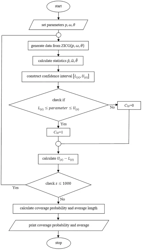
Figure 2:A flowchart of the simulation study

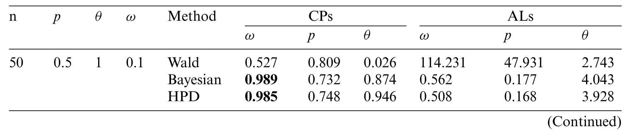
Table 2:The coverage probabilities and average lengths of the 95%confidence interval for parameters of the ZICG distribution

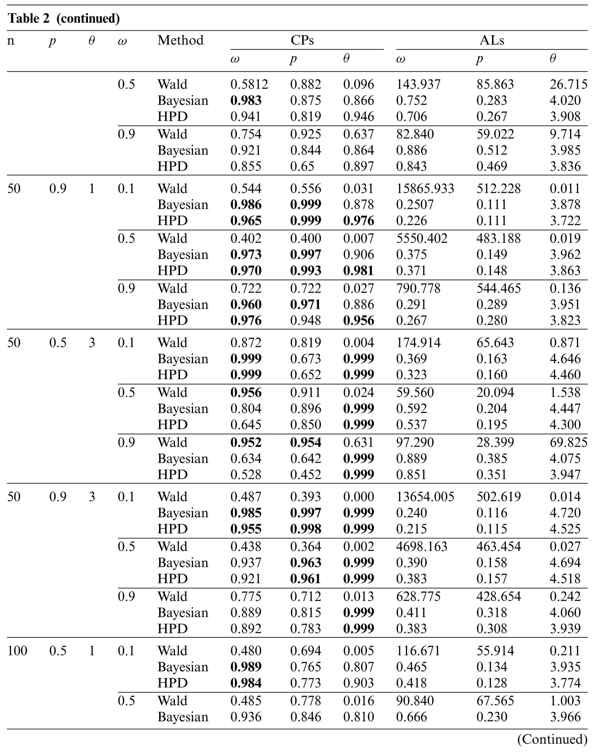
Table 2 (continued)npθωMethodCPsALs ωpθωpθ 0.5Wald0.58120.8820.096143.93785.86326.715 Bayesian0.9830.8750.8660.7520.2834.020 HPD0.9410.8190.9460.7060.2673.908 0.9Wald0.7540.9250.63782.84059.0229.714 Bayesian0.9210.8440.8640.8860.5123.985 HPD0.8550.650.8970.8430.4693.836 500.910.1Wald0.5440.5560.03115865.933512.2280.011 Bayesian0.9860.9990.8780.25070.1113.878 HPD0.9650.9990.9760.2260.1113.722 0.5Wald0.4020.4000.0075550.402483.1880.019 Bayesian0.9730.9970.9060.3750.1493.962 HPD0.9700.9930.9810.3710.1483.863 0.9Wald0.7220.7220.027790.778544.4650.136 Bayesian0.9600.9710.8860.2910.2893.951 HPD0.9760.9480.9560.2670.2803.823 500.530.1Wald0.8720.8190.004174.91465.6430.871 Bayesian0.9990.6730.9990.3690.1634.646 HPD0.9990.6520.9990.3230.1604.460 0.5Wald0.9560.9110.02459.56020.0941.538 Bayesian0.8040.8960.9990.5920.2044.447 HPD0.6450.8500.9990.5370.1954.300 0.9Wald0.9520.9540.63197.29028.39969.825 Bayesian0.6340.6420.9990.8890.3854.075 HPD0.5280.4520.9990.8510.3513.947 500.930.1Wald0.4870.3930.00013654.005502.6190.014 Bayesian0.9850.9970.9990.2400.1164.720 HPD0.9550.9980.9990.2150.1154.525 0.5Wald0.4380.3640.0024698.163463.4540.027 Bayesian0.9370.9630.9990.3900.1584.694 HPD0.9210.9610.9990.3830.1574.518 0.9Wald0.7750.7120.013628.775428.6540.242 Bayesian0.8890.8150.9990.4110.3184.060 HPD0.8920.7830.9990.3830.3083.939 1000.510.1Wald0.4800.6940.005116.67155.9140.211 Bayesian0.9890.7650.8070.4650.1343.935 HPD0.9840.7730.9030.4180.1283.774 0.5Wald0.4850.7780.01690.84067.5651.003 Bayesian0.9360.8460.8100.6660.2303.966(Continued)

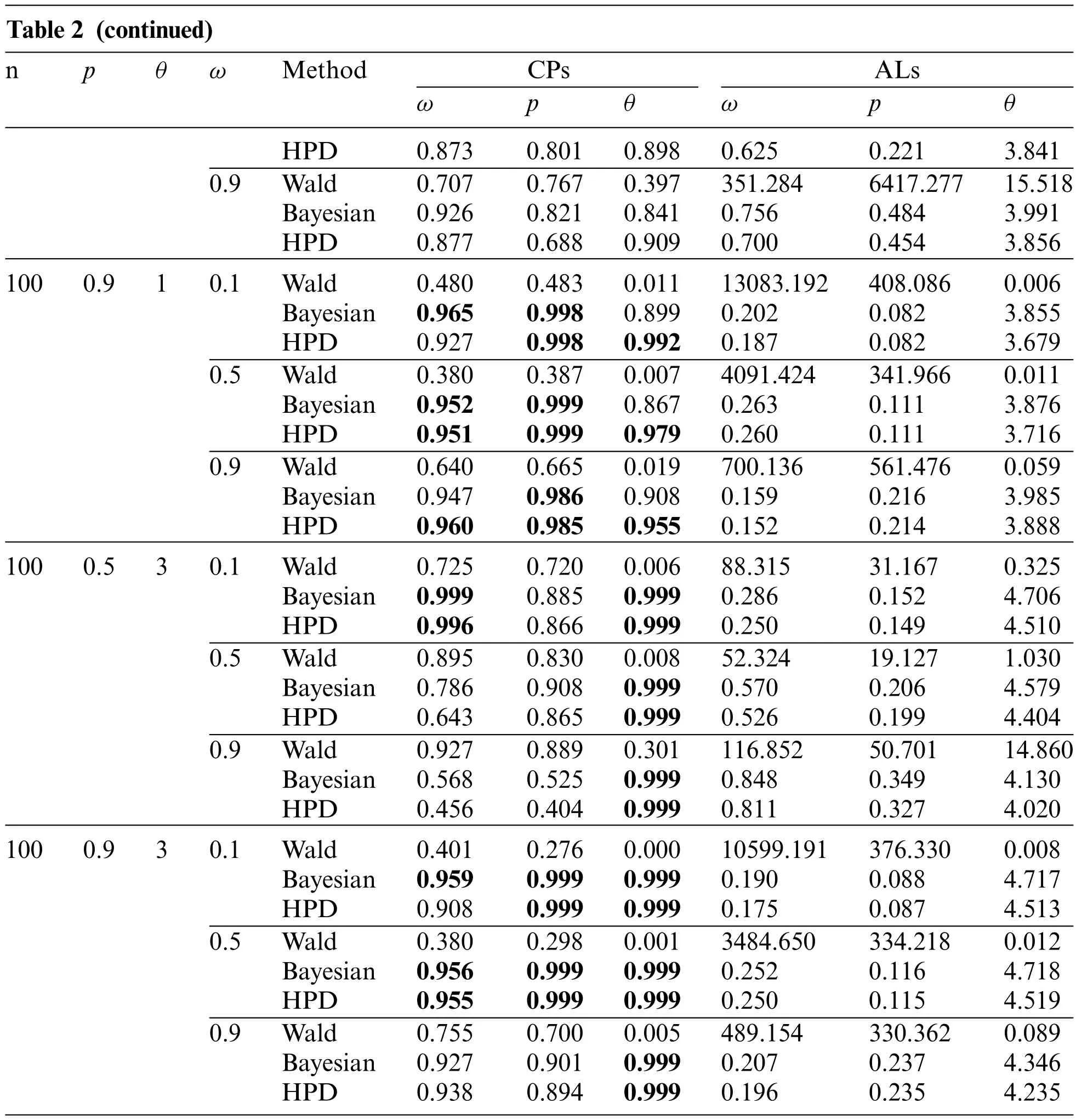
Table 2 (continued)npθωMethodCPsALs ωpθωpθ HPD0.8730.8010.8980.6250.2213.841 0.9Wald0.7070.7670.397351.2846417.27715.518 Bayesian0.9260.8210.8410.7560.4843.991 HPD0.8770.6880.9090.7000.4543.856 1000.910.1Wald0.4800.4830.01113083.192408.0860.006 Bayesian0.9650.9980.8990.2020.0823.855 HPD0.9270.9980.9920.1870.0823.679 0.5Wald0.3800.3870.0074091.424341.9660.011 Bayesian0.9520.9990.8670.2630.1113.876 HPD0.9510.9990.9790.2600.1113.716 0.9Wald0.6400.6650.019700.136561.4760.059 Bayesian0.9470.9860.9080.1590.2163.985 HPD0.9600.9850.9550.1520.2143.888 1000.530.1Wald0.7250.7200.00688.31531.1670.325 Bayesian0.9990.8850.9990.2860.1524.706 HPD0.9960.8660.9990.2500.1494.510 0.5Wald0.8950.8300.00852.32419.1271.030 Bayesian0.7860.9080.9990.5700.2064.579 HPD0.6430.8650.9990.5260.1994.404 0.9Wald0.9270.8890.301116.85250.70114.860 Bayesian0.5680.5250.9990.8480.3494.130 HPD0.4560.4040.9990.8110.3274.020 1000.930.1Wald0.4010.2760.00010599.191376.3300.008 Bayesian0.9590.9990.9990.1900.0884.717 HPD0.9080.9990.9990.1750.0874.513 0.5Wald0.3800.2980.0013484.650334.2180.012 Bayesian0.9560.9990.9990.2520.1164.718 HPD0.9550.9990.9990.2500.1154.519 0.9Wald0.7550.7000.005489.154330.3620.089 Bayesian0.9270.9010.9990.2070.2374.346 HPD0.9380.8940.9990.1960.2354.235

3.2 Applicability of the Methods When Using Real COVID-19 Data

Data for new daily COVID-19 cases during the Tokyo 2020 Olympic Games from 01 July 2021 to 12 August 2021 were used for this demonstration.The data are reported by the Tokyo Organizing Committee on the Government website (https://olympics.com/en/olympic-games/tokyo-2020) and they are shown in Table 3,with a histogram of the data provided in Fig.3.

Table 3: The number of daily COVID-19-positive cases during the olympic games in Tokyo 2020

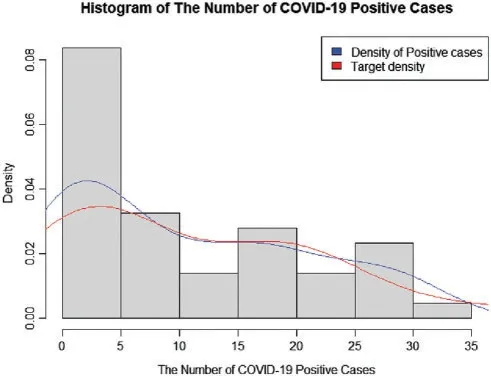
Figure 3:A histogram of the number of COVID-19-positive case during the olympic games in Tokyo 2020

3.2.1 Analysis of the COVID-19 Data

The information in Table 4 shows that the data are over-dispersed with an index of dispersion of 9.7149.The suitability of fitting the data to ZICG,ZIG,ZIP,ZINB,CG,geometric,Poisson,NB,and Gaussian distributions was assessed by using the AIC computed as AIC=2k−and the corrected AIC(AICc)computed as AICc=AIC+2k(k+1)/(n−k−1)based on the log-likelihood functionwherekis the number of parameters to fit.As can be seen in Table 5,the AIC and AICc values for ZICG were very similar (290.1166 and 290.7320) and the lowest recorded,thereby inferring that it provided the best fit for the data.

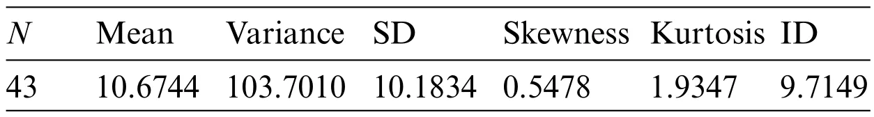
Table 4: Descriptive statistics

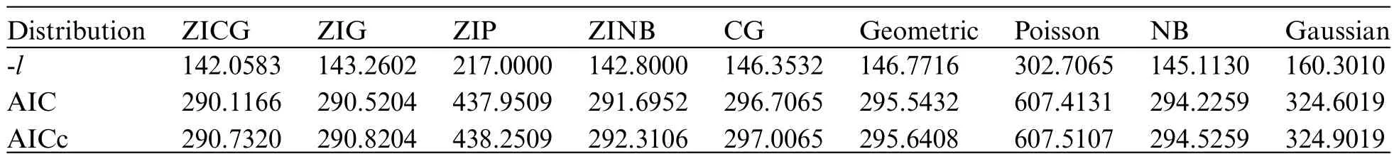
Table 5: Log-likelihood(l),AIC,and AICc values

The 95%confidence intervals for the parameters of a ZICG distribution constructed by using the three estimation methods are provided in Table 6.The maximum likelihood estimates for parametersω,p,andθwere 0.0743,0.9238,and 0.4967,respectively.From the simulation results in Table 2 forn=50,ω=0.1,p=0.9,andθ=1,the HPD intervals provided a coverage probability greater than 0.95 for all of the parameters.Hence the HPD intervals are recommended for constructing the 95%confidence intervals for the parameters in this scenario.

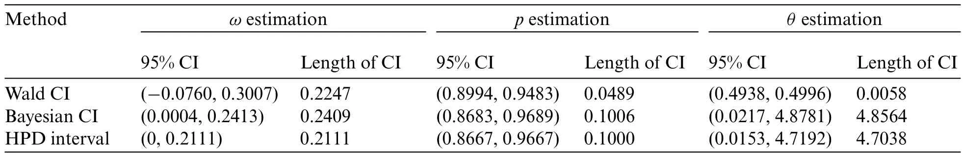
Table 6: Estimation of the number of daily COVID-19-positive cases during the olympic games in Tokyo 2020

4 Conclusions

We proposed a new mixture distribution called ZICG and presented its properties,namely the mgf,mean,variance,and Fisher information.According to the empirical study results,the ZICG distribution is suitable for over-dispersed count data containing excess zeros,such as occurred in the number of daily COVID-19-positive cases at the Tokyo 2020 Olympic Games.Confidence intervals for the three parameters of the ZICG distribution were constructed by using the Wald confidence interval,the Bayesian credible interval,and the HPD interval.Since the maximum likelihood estimates of the ZICG model parameters have no closed form,the Newton-Raphson method was applied to estimate the parameters and construct the Wald confidence intervals.Furthermore,Gibbs’sampling with the RWM algorithm was utilized in the Bayesian computation to approximate the parameters and construct the Bayesian credible intervals and the HPD intervals.Their performances were compared in terms of coverage probabilities and average lengths.According to the simulation results,the index of dispersion plays an important role:when it was small(e.g.,p=0.5),the Bayesian credible intervals and HPD intervals provided coverage probabilities greater than the nominal confidence level(0.95)in some cases whereas the Wald confidence interval did not perform at all well except for one case.Therefore,the Wald confidence interval approach is not recommended for constructing the confidence intervals for the ZICG parameters.Overall,the HPD interval approach is recommended for constructing the 95% confidence intervals for the parameters of a ZICG distribution since it provided coverage probabilities close to the nominal confidence level and the smallest average lengths in most cases.However,there are some cases where none of the methods performed well and so,in future research,other methods for estimating the parameters of a ZICG distribution will be investigated.For example,the prior part of the Bayesian computation should be further investigated to improve the efficiency of the Bayesian analysis.Furthermore,count data with more than one inflated value such as zeros-andones can occur,and so the zero-and-one inflated CG distribution could be interesting in this case.

Acknowledgement: The first author acknowledges the generous financial support from the Science Achievement Scholarship of Thailand(SAST).

Funding Statement:This research has received funding support from the National Science,Research and Innovation Fund(NSRF),and King Mongkut’s University of Technology North Bangkok(Grant No.KMUTNB-FF-65-22).

Conflicts of Interest:The authors declare that they have no conflicts of interest to report regarding the present study.

Appendix A.R code for simulation study

rCGD<−function(n,p,theta){

X=rep(0,n)

for(j in 1:n){

i=0

#step 1:Generated Uniform(0,1)

U=runif(1,0,1)

#step 2:Computed F(k∗−1)and F(k∗)

cdf<−(2 ∗(1−p)∗(1−2 ∗p ∗cos(2 ∗theta)+p∧2))

/(2+p ∗((p−3)∗cos(2 ∗theta)+p−1))

while(U>=cdf)

{i=i+1;

cdf=cdf+f(i,p,theta)}

X[j]=i;

}

return(X)

}

C<−function(p,theta){

(2 ∗(1−p)∗(1−2 ∗p ∗cos(2 ∗theta)+p∧2))/(2+p ∗((p−3)∗cos(2 ∗theta)+p−1))}

#Calculating log likelihood of CG

loglikeCG<−function(x,y){

p<−x[1]

theta<−x[2]

loglike<−n ∗log(2)+n ∗log(1−p)+

n ∗log(1−2 ∗p ∗cos(2 ∗theta)+p∧2)−

n ∗log(2+p ∗((p−3)∗cos(2 ∗theta)+p−1))+

log(p)∗sum(y)+2 ∗sum(log(cos(y ∗theta)))

#note use of sum

loglike<−−loglike

}

#Calculating the log-likelihood for ZICG

loglikeZICG<−function(x,y){

w<−x[1]

p<−x[2]

theta<−x[3]

n0<−length(y[which(y==0)])

ypos<−y[which(y!=0)]#y>0

loglike<−n0 ∗log(w+(1−w)∗C(p,theta))

+sum(log((1−w)∗C(p,theta)∗

(p∧ypos)∗cos(ypos ∗theta)∧2))

loglike<−−loglike

}

#Bayesian Confidence Interval

gibbs<−function(y=y,sample.size,n,p,theta,w){

nonzero_values=y[which(y!=0)]

m<−n−length(nonzero_values)

ypos=y[which(y!=0)]

prob.temp=numeric()

S.temp=numeric()

theta.temp=numeric(sample.size)

w.temp=numeric(sample.size)

p.temp=numeric(sample.size)

p.temp[1]<−0.5#initial p value

theta.temp[1]<−0.5#initial theta

w.temp[1]<−0.5#initial w value

prob.temp[1]<−w.temp[1]/(w.temp[1]+(1−w.temp[1])∗(2 ∗(1−p.temp[1])

∗1−2 ∗p.temp[1]∗cos(2 ∗theta.temp[1])+p.temp[1]∧2))/(2+p.temp[1]∗((p.temp[1]−3)

∗cos(2 ∗theta.temp[1])+p.temp[1]−1)))

S.temp[1]<−rbinom(1,m,prob.temp[1])

w.temp[1]<−rbeta(1,S.temp[1]+0.5,n−S.temp[1]+0.5)

p.samp<−GenerateMCMC.p(y=y,N=1000,n=n,m=m,w=w.temp[1],theta=theta.temp[1],

sigma=1)

p.temp[1]<−mean(p.samp[501:1000])

theta.samp<−GenerateMCMCsample(ypos=ypos,N=1000,n=n,m=m,w=w.temp[1],p=p.temp[1],

sigma=1)

theta.temp[1]<−mean(theta.samp[501:1000])

for(i in 2:(sample.size)){

prob.temp[i]<−w.temp[i−1]/(w.temp[i−1]+(1−w.temp[i−1])∗C(p.temp[i−1],

theta.temp[i−1]))

S.temp[i]<−rbinom(1,m,prob.temp[i])

w.temp[i]<−rbeta(1,S.temp[i]+0.5

,n−S.temp[i]+0.5)

p.samp<−GenerateMCMC.p(y=y,N=1000,n=n,m=m,w=w.temp[i],

theta=theta.temp[i−1],sigma=1)

p.temp[i]<−mean(p.samp[501:1000])

theta.samp<−GenerateMCMCsample(ypos=ypos,N=1000,n=n,m=m,w=w.temp[i],

p=p.temp[i],sigma=1)

theta.temp[i]<−mean(theta.samp[501:1000])}

return(cbind(w.temp,p.temp,theta.temp))}

#random walk Metropolis for sample theta

GenerateMCMCsample<−function(ypos,N,n,m,w,p,sigma){

prior<−function(x)dgamma(x,shape=2,rate=1/3)

theta.samp<−numeric(length=N)

theta.samp[1]<−runif(n=1,min=0,max=5)

for(j in 2:N){

Yj<−theta.samp[j−1]+rnorm(n=1,mean=0,sigma)

if(0<=Yj&&Yj<=pi/2){

alpha.cri<−((w+(1−w)∗C(p,Yj))∧m ∗((1−w)∗(2 ∗(1−p)∗(1−2 ∗p ∗cos(2 ∗Yj)+p∧2))/

(2+p ∗((p−3)∗cos(2 ∗Yj)+p−1)))∧(n−m)∗prod((cos(ypos ∗Yj))∧2)∗prior(Yj))/

((w+(1−w)∗C(p,theta.samp[j−1]))∧m ∗((1−w)∗(2 ∗(1−p)∗

(1−2 ∗p ∗cos(2 ∗theta.samp[j−1])+p∧2))/

(2+p ∗((p−3)∗cos(2 ∗theta.samp[j−1])+p−1)))∧(n−m)∗

prod((cos(ypos ∗theta.samp[j−1]))∧2)∗prior(theta.samp[j−1]))

}else{alpha.cri<−0}

U<−runif(1)

if(is.na(alpha.cri)){theta.samp[j]<−theta.samp[j−1]}else{

if(U

{theta.samp[j]<−Yj

}elsetheta.samp[j]<−theta.samp[j−1]}

}return(theta.samp)}

##Random Walk Metropolis sampler for p

GenerateMCMC.p<−function(y,N,n,m,w,theta,sigma){

prior<−function(x)dbeta(x,shape1=2,

shape2=5)

p.samp<−numeric(length=N)

p.samp[1]<−runif(n=1,min=0,max=1)

for(j in 2:N){

Yj<−p.samp[j−1]+rnorm(n=1,mean=0,sigma)

if(0<=Yj&&Yj<=1){

alpha.cri<−((w+(1−w)∗C(Yj,theta))∧m ∗((1−w)∗C(Yj,theta))∧(n−m)∗Yj∧(sum(y)))

∗prior(Yj)/((w+(1−w)∗C(p.samp[j−1],theta))∧m ∗

((1−w)∗C(p.samp[j−1],theta))∧(n−m)∗p.samp[j−1]∧(sum(y)))∗prior(p.samp[j−1])

}else{alpha.cri<−0}

U<−runif(1)

if(is.na(alpha.cri)){

p.samp[j]<−p.samp[j−1]}

else{if(U

p.samp[j]<−Yj

}elsep.samp[j]<−p.samp[j−1]}}

return(p.samp)

}

i=0

while(i

suscept<−rbinom(n,size=1,prob=1−w)

count<−rCGD(n,p,theta)

y=suscept ∗count

if(max(y)==0){

next

}i=i+1

p_hat<−egeom(y,method=“mle”)

p0=p_hat$parameters;theta0=0.5;

#store starting values

intvalues1=c(p0,theta0)

resultCG<−nlm(loglikeCG,intvalues1,y,hessian=TRUE,print.level=1)

mleCG<−resultCG$estimate

mleCG.p<−c(mleCG[1])

mleCG.theta<−c(mleCG[2])

#formula for estimating w(omega)

n0<−length(y[which(y==0)])

p1=mleCG.p;theta1=mleCG.theta;

c_hat<−C(p1,theta1)

w1<−(n0−n ∗c_hat)/(n ∗(1−c_hat))

intvalues2=c(w1,p1,theta1)

resultZICG<−nlm(loglikeZICG,intvalues2,y,hessian=TRUE,print.level=1)

mleZICG<−resultZICG$estimate

hess<−resultZICG$hessian

cov<−solve(hess,tol=NULL)

stderr<−sqrt(diag(cov))

mle.w<−c(mleZICG[1])

mle.p<−c(mleZICG[2])

mle.theta<−c(mleZICG[3])

sd.w<−stderr[1]

sd.p<−stderr[2]

sd.theta<−stderr[3]

#Wald confidence interval for w

#lower bound of Wald CI for w

Wald.w.L[i]<−mle.w−qnorm(1−alpha/2)∗sd.w

#Upper bound of Wald CI for w

Wald.w.U[i]<−mle.w+qnorm(1−alpha/2)∗sd.w

Wald.CI.w=rbind(c(Wald.w.L[i],Wald.w.U[i]))

Wald.CP.w[i]=ifelse(Wald.w.L[i]

Wald.Length.w[i]=Wald.w.U[i]−Wald.w.L[i]

#Wald confidence interval for p

#lower bound of Wald CI for p

Wald.p.L[i]<−mle.p−qnorm(1−alpha/2)∗sd.p

#Upper bound of Wald CI for p

Wald.p.U[i]<−mle.p+qnorm(1−alpha/2)∗sd.p

Wald.CI.p=rbind(c(Wald.p.L[i],Wald.p.U[i]))

Wald.CP.p[i]=ifelse(Wald.p.L[i]

Wald.Length.p[i]=Wald.p.U[i]−Wald.p.L[i]

#Wald confidence interval for theta

#lower bound of Wald CI for theta

Wald.theta.L[i]<−mle.theta−qnorm(1−alpha/2)∗sd.theta

#Upper bound of Wald CI for theta

Wald.theta.U[i]<−mle.theta+qnorm(1−alpha/2)∗sd.theta

Wald.CI.theta=rbind(c(Wald.theta.L[i],Wald.theta.U[i]))

Wald.CP.theta[i]=ifelse(Wald.theta.L[i]

Wald.Length.theta[i]=Wald.theta.U[i]−Wald.theta.L[i]

#########End Wald CI#############

test<−gibbs(y=y,sample.size=sample.size,

n=n,p=p,theta=theta,w=w)

#burn-in w estimator

w.mcmc<−test[,1][1001:3000]

#estimator of w

w.bayes<−mean(w.mcmc)

#burn-in p estimator

p.mcmc<−test[,2][1001:3000]

#estimator of p

p.bayes<−mean(p.mcmc)

#burn-in theta estimator

theta.mcmc<−test[,3][1001:3000]

#estimator of theta

theta.bayes<−mean(theta.mcmc)

#########Construct Bayesian confidence interval########

L.w[i]=quantile(w.mcmc,alpha/2,na.rm=TRUE)

U.w[i]=quantile(w.mcmc,(1−alpha/2),na.rm=TRUE)

CIr1=rbind(c(L.w[i],U.w[i]))

Bayes.CP.w[i]=ifelse(L.w[i]

Bayes.Length.w[i]=U.w[i]−L.w[i]

L.p[i]=quantile(p.mcmc,alpha/2,na.rm=TRUE)

U.p[i]=quantile(p.mcmc,(1−alpha/2),na.rm=TRUE)

CIr2=rbind(c(L.p[i],U.p[i]))

Bayes.CP.p[i]=ifelse(L.p[i]

Bayes.Length.p[i]=U.p[i]−L.p[i]

L.the[i]=quantile(theta.mcmc,alpha/2,na.rm=TRUE)

U.the[i]=quantile(theta.mcmc,(1−alpha/2),na.rm=TRUE)

CIr3=rbind(c(L.the[i],U.the[i]))

Bayes.CP.the[i]=ifelse(L.the[i]

Bayes.Length.the[i]=U.the[i]−L.the[i]

#########Construct HPD interval########

w.hpd=hdi(w.mcmc,0.95)

L.w.hpd[i]=w.hpd[1]

U.w.hpd[i]=w.hpd[2]

CIr4=rbind(c(L.w.hpd[i],U.w.hpd[i]))

CP.w.hpd[i]=ifelse(L.w.hpd[i]

Length.w.hpd[i]=U.w.hpd[i]−L.w.hpd[i]

p.hpd=hdi(p.mcmc,0.95)

L.p.hpd[i]=p.hpd[1]

U.p.hpd[i]=p.hpd[2]

CIr5=rbind(c(L.p.hpd[i],U.p.hpd[i]))

CP.p.hpd[i]=ifelse(L.p.hpd[i]

Length.p.hpd[i]=U.p.hpd[i]−L.p.hpd[i]

theta.hpd=hdi(theta.mcmc,0.95)

L.the.hpd[i]=theta.hpd[1]

U.the.hpd[i]=theta.hpd[2]

CIr6=rbind(c(L.the.hpd[i],U.the.hpd[i]))

CP.the.hpd[i]=ifelse(L.the.hpd[i]

Length.the.hpd[i]=U.the.hpd[i]−L.the.hpd[i]

}