
A New Three-Parameter Inverse Weibull Distribution with Medical and Engineering Applications
2023-02-26 10:17RefahAlotaibiHassanOkashaHodaRezkandMazenNassar
Refah Alotaibi,Hassan Okasha,Hoda Rezk and Mazen Nassar
1Department of Mathematical Sciences,College of Science,Princess Nourah bint Abdulrahman University,Riyadh,11671,Saudi Arabia
2Department of Statistics,Faculty of Science,King Abdulaziz University,Jeddah,21589,Saudi Arabia
3Department of Mathematics,Faculty of Science,Al-Azhar University,Nasr City,11884,Cairo,Egypt
4Department of Statistics,Faculty of Commerce,Al-Azhar University,Nasr City,11884,Cairo,Egypt
5Department of Statistics,Faculty of Commerce,Zagazig University,Zagazig,44519,Egypt
ABSTRACT The objective of this article is to provide a novel extension of the conventional inverse Weibull distribution that adds an extra shape parameter to increase its flexibility.This addition is beneficial in a variety of fields,including reliability,economics,engineering,biomedical science,biological research,environmental studies,and finance.For modeling real data,several expanded classes of distributions have been established.The modified alpha power transformed approach is used to implement the new model.The data matches the new inverse Weibull distribution better than the inverse Weibull distribution and several other competing models.It appears to be a distribution designed to support decreasing or unimodal shaped distributions based on its parameters.Precise expressions for quantiles,moments,incomplete moments,moment generating function,characteristic generating function,and entropy expression are among the determined attributes of the new distribution.The point and interval estimates are studied using the maximum likelihood method.Simulation research is conducted to illustrate the correctness of the theoretical results.Three applications to medical and engineering data are utilized to illustrate the model’s flexibility.
KEYWORDS Inverse weibull distribution;modified alpha power transformation method;moments;order statistics
1 Introduction
Recently,many statistical distributions have been proposed by statisticians.The necessity to develop new distributions appear either due to practical investigations or theoretical concerns or both.Many applications in domains including dependability analysis,finance and risk modelling,insurance,and biological sciences,among others,have indicated in recent years that data sets that follow standard distributions are more often the exception than the usual.Because modified distributions are necessary,significant progress has been made in the modification of several classic distributions and their efficient utilization to challenges in these fields.Lately,specifically since 1980,the direction of statisticians to develop new distributions is on adding parameter(s)to some existing distributions or integrating classical distributions,see Lee et al.[1].This addition of parameter(s) has been demonstrated valuable in analysing tail properties and also for enhancing the goodness of fit of the family under consideration.For more details about the methods of adding parameters,one can refer to Mudholkar et al.[2],Marshall et al.[3]and Mahdavi et al.[4].
The inverse-Weibull (IW) distribution has many vital applications in life testing and reliability studies.The IW distribution bears some other names like Fréchet distribution.The IW distribution is viewed as reciprocal to the usual Weibull distribution,see Drapella[5]and Mudholkar et al.[6],it is used to describe the degradation of mechanical components in diesel engines,such as the crankshaft and pistons,see Keller et al.[7].Several academics proposed several modified variations of the IW distribution to increase its flexibility.Khan[8]looked at the beta IW distribution,for example.The generalized IW distribution was proposed by de Gusmao et al.[9],the modified IW distribution was proposed by Khan et al.[10],the Kumaraswamy generalized IW distribution was proposed by Oluyede et al.[11],and the Kumaraswamy modified IW distribution was proposed by Aryal et al.[12].In addition,Okasha et al.[13]suggested the Marshall-Olkin IW distribution,Basheer[14]proposed the alpha power IW distribution,Dey et al.[15]discussed the logarithmic transformed IW distribution,and Afify et al.[16]suggested the logarithmic transformed IW distribution.
Assume thatXis a random variable follows IW distribution withδas the scale parameter andθas the shape parameter,whereδ,θ >0.Then,the probability density function(PDF)ofXcan be written as follows:
The cumulative distribution function(CDF)of Eq.(1)is
See Johnson et al.[17]for further information on the IW distribution.In this study,we offer a new three-parameter IW distribution utilizing the same idea proposed by Alotaibi et al.[18].The modified alpha power transformed IW(MAPTIW)distribution is the name given to the new distribution.Two shape parameters and one scale parameter are included.It includes some lifetime distributions,such as IW,inverted exponential and inverse Rayleigh distributions.Recently,The alpha power transformation approach was used by Alotaibi et al.[18]to suggest a new method for adding a new shape parameter to a baseline distribution.Modified alpha power transformation(MAPT)was the name given to the approach they proposed.The CDF and PDF of MAPT method are expressed as
and
whereαis a new shape parameter.This article seeks to furnish a new lifetime model with the lowest number of parameters,yet satisfactory to depict more complicated data patterns; one scale and two shape parameters are involved to accommodate for decreasing and upside-down bathtubshaped failure rates.The MAPTIW distribution is motivated by the following causes: (1) It is a comprehensive distribution that holds some well-known lifetime distributions.(2) It is established in Section 2 that the MAPTIW distribution can be considered as a mixture of the traditional IW distribution.(3)The MAPTIW distribution can deliver decreasing and unimodal hazard rates which makes it outstanding from some other distributions.(4)The MAPTIW can be viewed as a practical model for modelling skewed data which can not be adequately modelled by other distributions.(5)The MAPTIW distribution furnishes more significant flexibility when compared with many well-known distributions in two real data applications.We seek that it will attract wider applications in medicine,engineering and other fields of research.
The remainder of this article is structured as follows.The MAPTIW distribution is introduced and its mixed representation is derived in Section 2.In Section 3,we will look at some of the MAPTIW’s most important characteristics.Section 4 shows how to estimate unknown parameters using maximum likelihood estimation.We present the simulation results in Section 5 to show how well the estimations performed.Three real-life data sets are used to assess the importance of the MAPTIW distribution in Section 6.Section 7 presents the conclusion.
2 MAPTIW Distribution
We may define the CDF of the MAPTIW distribution in the following form by inserting the CDF of the IW distribution obtained by Eq.(2)into the CDF of the MAPT generator given by Eq.(3)
The PDF that corresponds to the CDF in Eq.(5)can be expressed as follows:
MAPTIW distribution has the following special sub-models.Ifα→1,it reduces to the IW distribution.Ifθ=1 andα→1,it reduces to the inverted exponential distribution.Ifθ=2 andα→1,it reduces to the inverse Rayleigh distribution.Also,whenθ=1,it reduces to the MAPT-inverted exponential distribution.Finally,whenθ=2,it simplifies to the MAPT-Rayleigh distribution.The MAPTIW distribution’s reliability function (RF) and hazard rate function (HRF)are
and
respectively.Henceforth,we will useXto refer to the random variable that possesses the PDF in Eq.(6).
The various plots of the PDF of the MAPTIW distribution withδ=1 in all settings and different values forαandθare shown in Fig.1.The newly introduced parameterαoffered more extra flexibility to the PDF of the MAPTIW distribution,as seen in Fig.1.The MAPTIW distribution is rightskewed,and because of this,it is more suited to modelling right-skewed data than other competing distributions.The many forms of the HRF of the MAPTIW distribution are shown in Fig.2.It shows that the MAPTIW distribution’s HRF can be decreasing or unimodal in form.
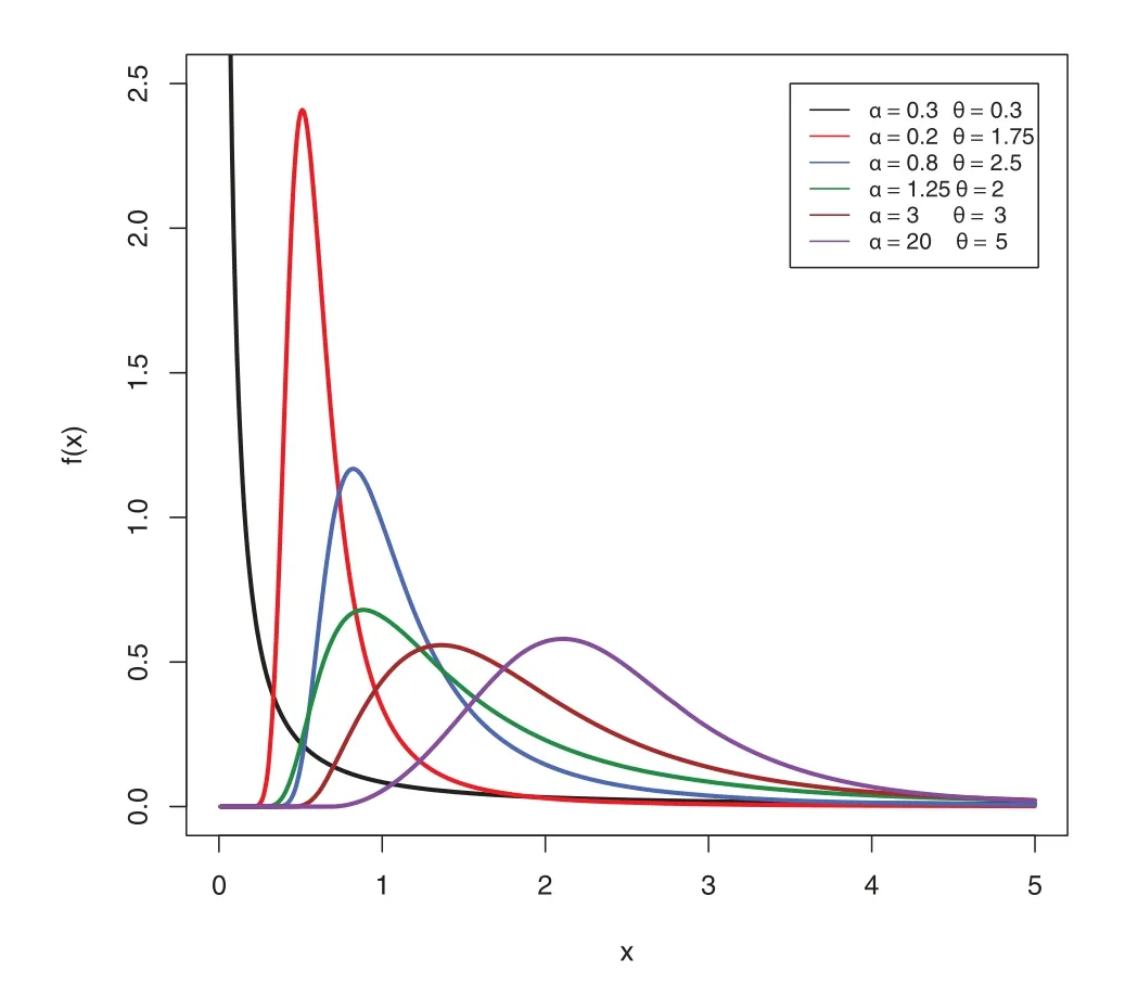
Figure 1:MAPTIW PDF plots

Figure 2:HRF plots for the MAPTIW distribution
The PDF in Eq.(6) might be used to obtain various statistical characteristics of the MAPTIW distribution.Finding the PDF’s mixture structure in Eq.(5) is a simple method.Observe the power series below:
whereyis a variable and log(α)is a constant,as well as the generalized binomial expansion,which has the form
whereyis a variable,ais a constant andΓ(a)is the gamma function defined asΓ(a)=
When Eqs.(9) and (10) are applied to the PDF in Eq.(6),the following is a suitable linear representation for the PDF
whereg(x;(m+1)δ,θ) is the PDF of the IW distribution with scale parameter(m+1)δand shape parameterθ,and
On the other hand,the expansion of the CDF in Eq.(5)may be provided as by integrating Eq.(11)as
HenceG(x;(m+1)δ,θ)is the CDF corresponding tog(x;(m+1)δ,θ).
3 MAPTIW Distribution’s Properties
The quantile function,moments and stress-strength parameter are some of the properties of the MAPTIW distribution that we derive in this part.
3.1 Quantile Function
The quantile function for the MAPTIW distribution may be calculated as follows using Eq.(5):
One can employ Eq.(13)to simulate the random variableXby takingu∼Uniform(0,1).
3.2 Moments
Moments play an essential part in statistics.Numerous vital aspects of any statistical distribution can be explored via moments.For the MAPTIW distribution,thenthmoment can be obtained as
whereΓ(.)is the gamma function.In particular,the first two moments can be obtained as
and
The following formulae can also be used to obtain the variance(var),skewness(Sk),and kurtosis(Ku):
and
whereμ=μ′1.The propositions that follow are an explanation of three different types of moments,namely,incomplete moments (IMs),moment generating function (MGF),characteristic generating function(CGF)and conditional moments(CMs).
Prop 3.1.IfX∼MAPTIW,then the IMs ofXis given as follows:
whereγ(.,.)is the incomplete gamma function.
Prop 3.2.IfX∼MAPTIW,then the MGF,denoted byM(t),and the cumulant generating function,denoted byK(t),ofXare,respectively,given by
Prop 3.3.IfX∼MAPTIW,then the CGF ofXis
Prop 3.4.IfX∼MAPTIW,then the CMs ofXis
whereψn(t)is thenthIM ofX.
3.3 Entropies of MAPTIW Distribution
Entropy is used to measure uncertainty.It recreates a vital role in the area of engineering,probability,statistics,information theory and financial analysis.For example,Gençay et al.[19]delivered a relative analysis of the stock market during the 1987 and 2008 financial crises.Rashidi et al.[20]examined and simulated the heat transfer flow employing entropy generation in solar still.The Rényi entropy(RE)for the MAPTIW distribution may be calculated using Eq.(6)as follows:
The Shannon entropy can also be calculated as
3.4 Order Statistics
LetX1,...,Xn be a MAPTIW random sample of sizen.Assume thatX(1),...,X(n) are the corresponding order statistics.Theithorder statistic’s PDF is then presented as follows:
The beta function is represented asB(.,.).Using Eqs.(5),(6)and after some simplifications,we can obtain
whereg(x;(l+ 1)δ,θ) is the PDF of the IW distribution with scale parameter(l+ 1)δand shape parameterθ,and
Using Eq.(17),we can derive the properties ofX(i)directly from the properties ofZ(l+1),whereZ(l+1)follows IW distribution with scale parameter(l+1)δand shape parameterθ.Also,theqthmoments ofX(i)can be derive as follows:
3.5 Moments of Residual Life and Reversed Failure Rate Function
The mean residual lifetime has been studied by engineers and survival analysts.Given a feature or a system is of aget,the remaining lifetime aftertis a random variable.The expected value of this random residual lifetime is named the mean residual life.The mean residual lifetime is often a significant measure for discovering an optimal burn-in time for a feature.Therthmoment of the residual life ofXis given by
Using Eqs.(5)and(6),and the binomial expansion of(x−t)r,we get
The mean residual lifetime can be obtained from the last equation by settingr=1.Therthmoment of the reversed residual lifetime can be obtained as follows:
Based on Eqs.(5),(6)and using the binomial expansion of(t−x)r,we can write
3.6 Stress-Strength Model
LetY1∼MAPTIW(α1,θ1,δ1) andY2∼MAPTIW(α2,θ2,δ2).IfY1describes the stress andY2describes the strength,then the MAPTIW distribution’s stress-strength parameter,indicated byR.It has a wide range of applications in engineering and research.We will concentrate on two different cases.
Case one:α1/=α2,δ1=δ2=δandθ1=θ2=θ
Using the series expansion in Eq.(10),it follows:
Using the series expansion in Eq.(9),we can obtain
where
Case two:α1/=α2,δ1/=δ2andθ1/=θ2
Using the series expansion in Eq.(10),we have
Using the series expansion in Eq.(9),we can obtain
4 Parameter Estimation
In this section,we consider the maximum likelihood approach to estimate the unknown parameters of the MAPTIW distribution.Furthermore,the approximate confidence intervals(ACIs)of the unknown parameters are acquired.
4.1 Maximum Likelihood Estimation
Given a random sample of sizentaken from the MAPTIW distribution with PDF given by Eq.(6),we can express the log-likelihood function as
The maximum likelihood estimates (MLEs) denoted by,andcan be got by solving the following normal equations simultaneously
where
and
To get the MLEs ofα,δandθ,any numerical technique can be used to solve Eqs.(21)–(23).Using the asymptotic properties of the MLEs,we can construct the ACIs ofα,δandθ.It is known t hatwhereI0−1(α,δ,θ)is the asymptotic variance-covariance of the MLEs.Here,we employ the approximate asymptotic variance-covariance matrix of the MLEs denoted bywhich obtained based on the observed Fisher information matrix to compute the ACIs as follows:
whereIαα,Iδα=Iαδ,Iαθ=Iθα,Iδθ=Iθδ,IδδandIθθare derived from Eq.(20)as
and
where
Therefore,the(1−γ)%ACIs ofα δ,andθare as follows:
wherezγ/2is the upper(γ/2)thpercentile point of a standard normal distribution.
5 Simulation Study
In this part,we use a simulation with variable sample sizesnand various values of the parametersα,δ,andθto show how well the MLEs of the MAPTIW distribution perform.The results are based on sample sizes of 20,50,and 100 with parameter valuesα=(1.5,3,5),δ=(0.5,1.5,3) andθ=(1.5,3,5),respectively.We get MLEs,mean square errors (MSEs),and confidence lengths (CLs) in each case.The simulation study is implemented using the steps below:
1.Establish the sample size and parameter initial values.
2.Create a random sample of sizenfrom the MAPTIW distribution using Eq.(13).
3.Compute the MLEs ofα,δandθ.
4.Compute the MSEs ofα,δandθ.
5.Get the CLs ofα,δandθ.
6.Redo Steps 2–5,1000 times.
7.Determine the average values of estimates(AEs),MSEs,and CLs as follows:
whereξis the unknown parameter andξjU,ξjLare the lower and upper confidence bounds,respectively.Tables 1–3 present the simulation results.We can see from these Tables that the AEs of the parameters tend to be the true parameter values as the sample size increases.As a result,the MLEs perform like asymptotically unbiased estimators.In all cases,the MSEs decrease as the sample size grows,indicating that the MLEs are consistent.In all situations,the CLs decrease as the sample size increases,as expected,because asnincreases,some new information is acquired.
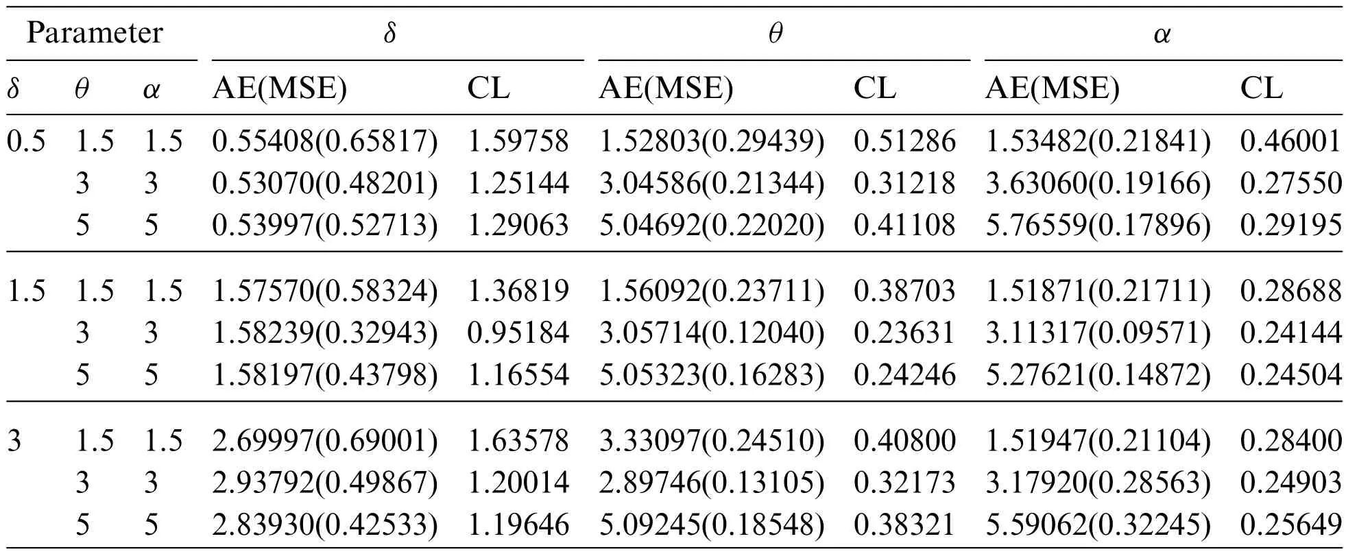
Table 1: AEs,MSEs(in parentheses)and CLs of the parameters at sample size,n=20
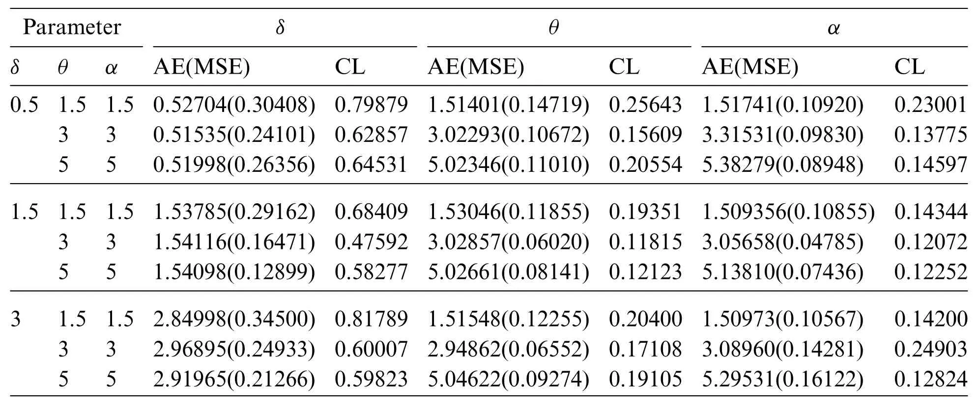
Table 2: AEs,MSEs(in parentheses)and CLs of the parameters at sample size,n=50
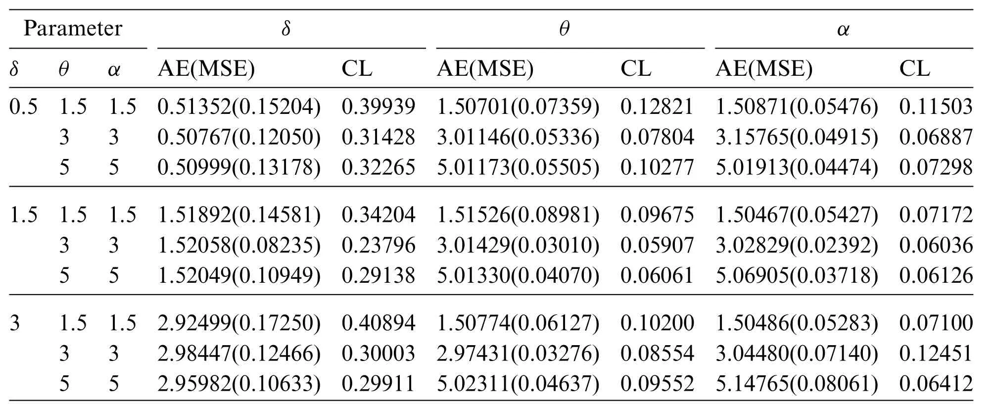
Table 3: AEs,MSEs(in parentheses)and CLs of the parameters at sample size,n=100
6 Applications
In this part,we illustrate the MAPTIW distribution’s flexibility by using three real data sets.The MAPTIW distribution is compared to other models such as,alpha power inverse Lomax(APILo)distribution by ZeinEldin et al.[21],inverse Lomax(ILo)distribution,alpha power inverse Weibull (APIW) distribution by Basheer [14],alpha power inverse Lindley (APILi) distribution by Dey et al.[22]and Weibull(We)distribution.Table 4 displays the PDFs of these distributions.
The first data(Data 1)describes the mortality rates due to the COVID-19 pandemic in the United Kingdom for 76 days,from 15 April to 30 June 2020.The data is originally investigated by Mubarak et al.[23].The entire data set is as follows: 0.0587,0.0863,0.1165,0.1247,0.1277,0.1303,0.1652,0.2079,0.2395,0.2751,0.2845,0.2992,0.3188,0.3317,0.3446,0.3553,0.3622,0.3926,0.3926,0.4110,0.4633,0.4690,0.4954,0.5139,0.5696,0.5837,0.6197,0.6365,0.7096,0.7193,0.7444,0.8590,1.0438,1.0602,1.1305,1.1468,1.1533,1.2260,1.2707,1.3423,1.4149,1.5709,1.6017,1.6083,1.6324,1.6998,1.8164,1.8392,1.8721,1.9844,2.1360,2.3987,2.4153,2.5225,2.7087,2.7946,3.3609,3.3715,3.7840,3.9042,4.1969,4.3451,4.4627,4.6477,5.3664,5.4500,5.7522,6.4241,7.0657,7.4456,8.2307,9.6315,10.187,11.1429,11.2019,11.4584.
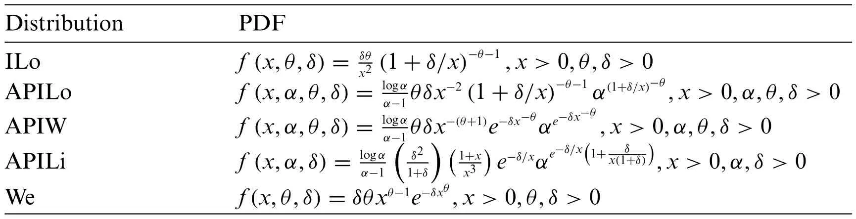
Table 4: The PDFs of different models
The second data set (Data 2) describes the remission times (in months) of a random sample of 128 bladder cancer patients studied by Lee et al.[24] and recently investigated by Al-Zahrani et al.[25–27].The complete data set of is: 0.08,2.09,3.48,4.87,6.94,8.66,13.11,23.63,0.20,2.23,3.52,4.98,6.97,9.02,13.29,0.40,2.26,3.57,5.06,7.09,9.22,13.80,25.74,0.50,2.46,3.64,5.09,7.26,9.47,14.24,25.82,0.51,2.54,3.70,5.17,7.28,9.74,14.76,26.31,0.81,2.62,3.82,5.32,7.32,10.06,14.77,32.15,2.64,3.88,5.32,7.39,10.34,14.83,34.26,0.90,2.69,4.18,5.34,7.59,10.66,15.96,36.66,1.05,2.69,4.23,5.41,7.62,10.75,16.62,43.01,1.19,2.75,4.26,5.41,7.63,17.12,46.12,1.26,2.83,4.33,5.49,7.66,11.25,17.14,79.05,1.35,2.87,5.62,7.87,11.64,17.36,1.40,3.02,4.34,5.71,7.93,11.79,18.10,1.46,4.40,5.85,8.26,11.98,19.13,1.76,3.25,4.50,6.25,8.37,12.02,2.02,3.31,4.51,6.54,8.53,12.03,20.28,2.02,3.36,6.76,12.07,21.73,2.07,3.36,6.93,8.65,12.63,22.69.
The third data set(Data 3)consists of the times of breakdown of a sample of 25 devices at 180°C and given by Pham[28].The complete data set of is:112,260,298,327,379,487,593,658,701,720,734,736,775,915,974,1123,1157,1227,1293,1335,1472,1529,1545,2029,4568.
Before studying these data sets,we foremost scheme the corresponding TTT plots.Fig.3 displays the TTT plots of these data.It indicates that Data 1 has a decreasing failure rate function,while the TTT plots for Data 2 and 3 reveal an upside-down bathtub failure rate function.Therefore,we can infer that the MAPTIW distribution is reasonable to model these data sets.The MLEs and their standard errors (SEs) of the MAPTIW distribution and some other competitive distributions are displayed in Tables 5,6 and 7 for Data 1,2 and 3,respectively.In addition,some goodness of fit statistics,namely,Akaike information criterion (AIC),consistent Akaike information criterion (CAIC),Bayesian information criterion (BIC),Hannan-Quinn information criterion (HQIC)statistics,Anderson-Darling(A),Cramér-Von Mises(W⋆)and Kolmogorov-Smirnov(K.S)(with the correspondingp-value)are also presented in Tables 5,6 and 7 for Data 1,2 and 3,respectively.It is noted from these Tables that the MAPTIW distribution performed better than all other competitive distributions.As a result,the MAPTIW distribution is determined to be the best model to fit the given two data sets.Figs.4–6 display the fitted PDFs,CDFs,RFs and probability-probability (PP) plots of the MAPTIW distribution for Data 1,2 and 3,respectively.These figures demonstrate that the MAPTIW distribution can furnish a close fit to the given data sets.Generally,we can deduce that the MAPTIW distribution is appropriate for modelling the delivered data sets more preferably than some conventional and some lately suggested models.The ACIs of the unknown parameters of the MAPTIW distribution for Data 1,2 and 3 are obtained and displayed in Table 8.
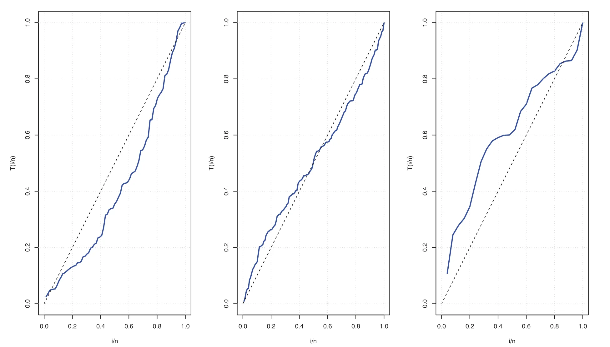
Figure 3:TTT Plots for Data 1(left)and Data 2(middle)and Data 3(right)
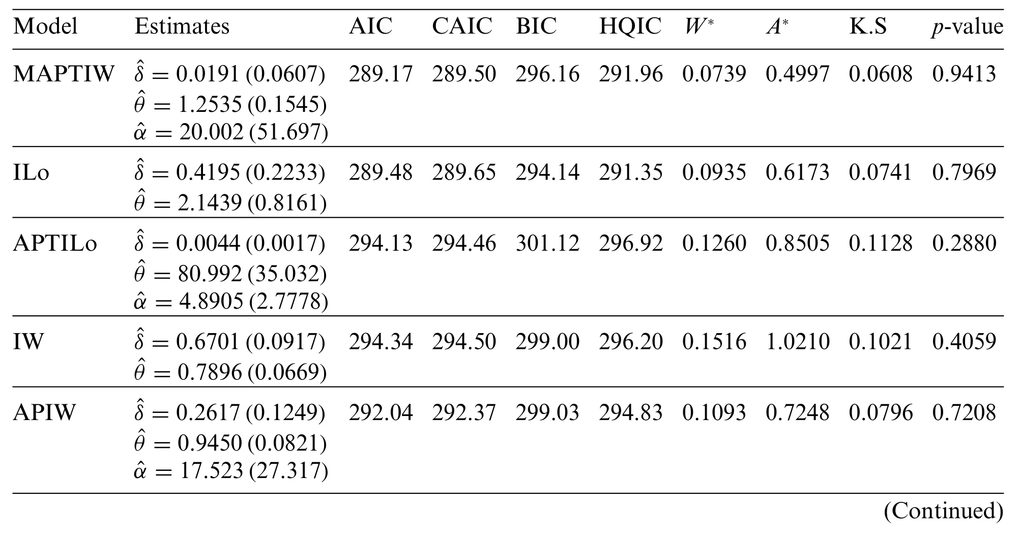
Table 5: MLEs,SEs(in parentheses)and different statistics for Data 1
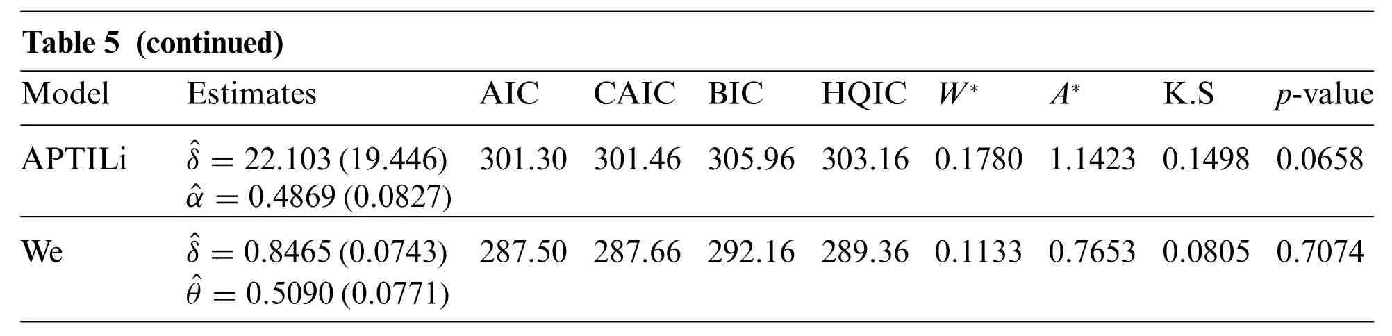
Table 5 (continued)ModelEstimatesAICCAIC BICHQIC W∗A∗K.Sp-value APTILiˆδ=22.103(19.446) 301.30 301.46 305.96 303.16 0.1780 1.1423 0.1498 0.0658 ˆα=0.4869(0.0827)Weˆδ=0.8465(0.0743) 287.50 287.66 292.16 289.36 0.1133 0.7653 0.0805 0.7074 ˆθ=0.5090(0.0771)
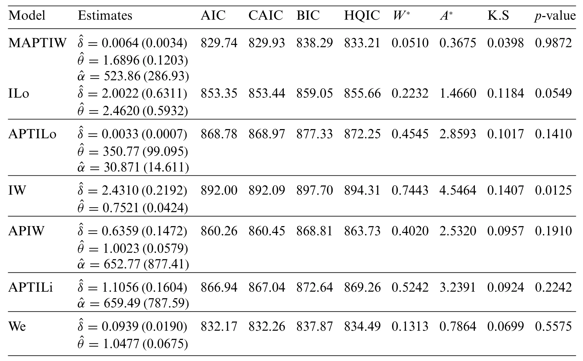
Table 6: MLEs,SEs(in parentheses)and different statistics for Data 2
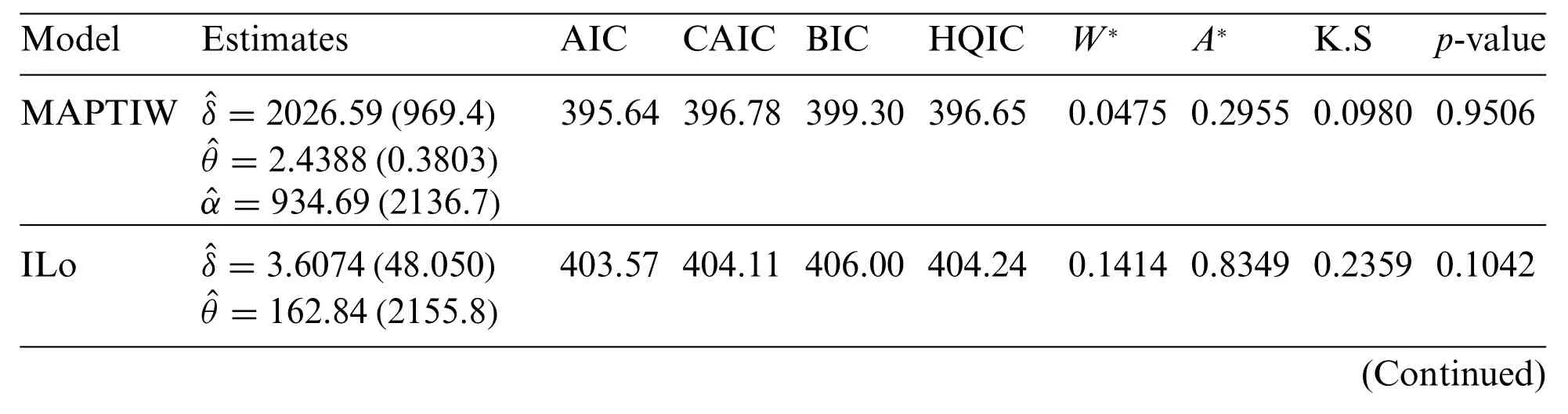
Table 7: MLEs,SEs(in parentheses)and different statistics for Data 3
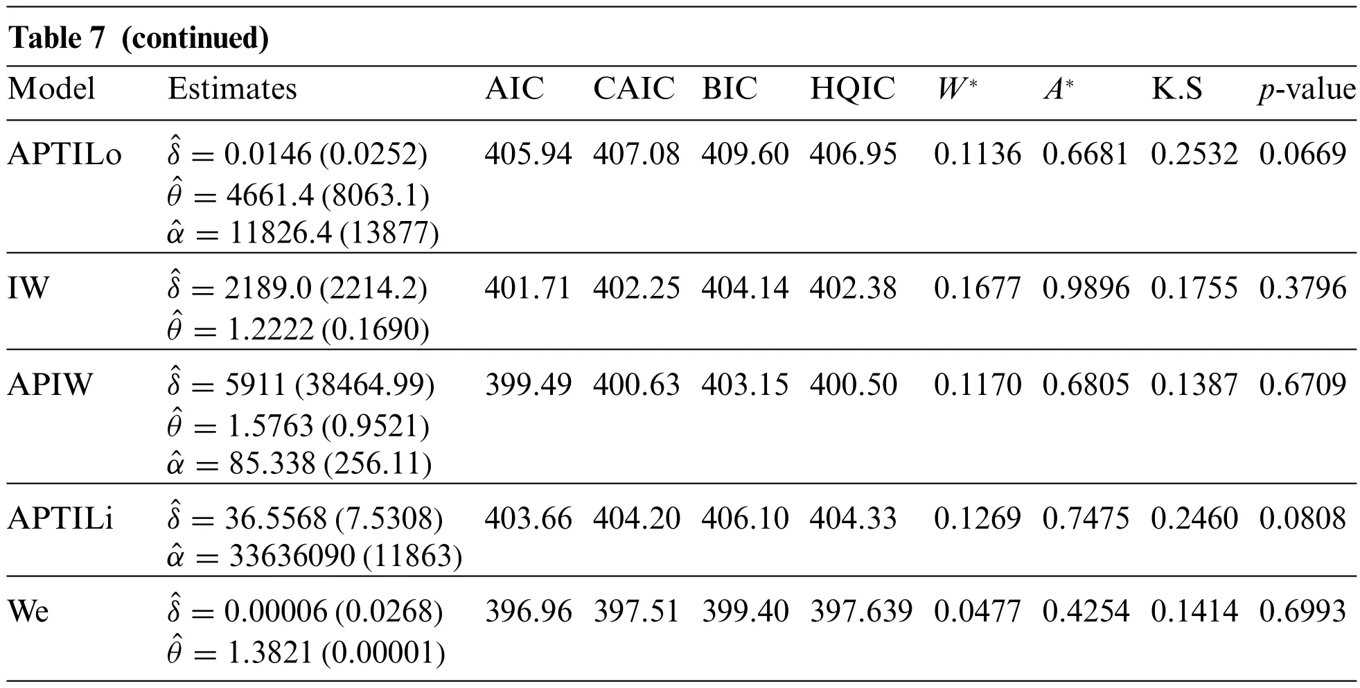
Table 7 (continued)ModelEstimatesAICCAIC BICHQIC W∗A∗K.Sp-value APTILoˆδ=0.0146(0.0252)405.94 407.08 409.60 406.95 0.1136 0.6681 0.2532 0.0669 ˆθ=4661.4(8063.1)ˆα=11826.4(13877)IWˆδ=2189.0(2214.2)401.71 402.25 404.14 402.38 0.1677 0.9896 0.1755 0.3796 ˆθ=1.2222(0.1690)APIWˆδ=5911(38464.99)399.49 400.63 403.15 400.50 0.1170 0.6805 0.1387 0.6709 ˆθ=1.5763(0.9521)ˆα=85.338(256.11)APTILiˆδ=36.5568(7.5308) 403.66 404.20 406.10 404.33 0.1269 0.7475 0.2460 0.0808 ˆα=33636090(11863)Weˆδ=0.00006(0.0268) 396.96 397.51 399.40 397.639 0.0477 0.4254 0.1414 0.6993 ˆθ=1.3821(0.00001)
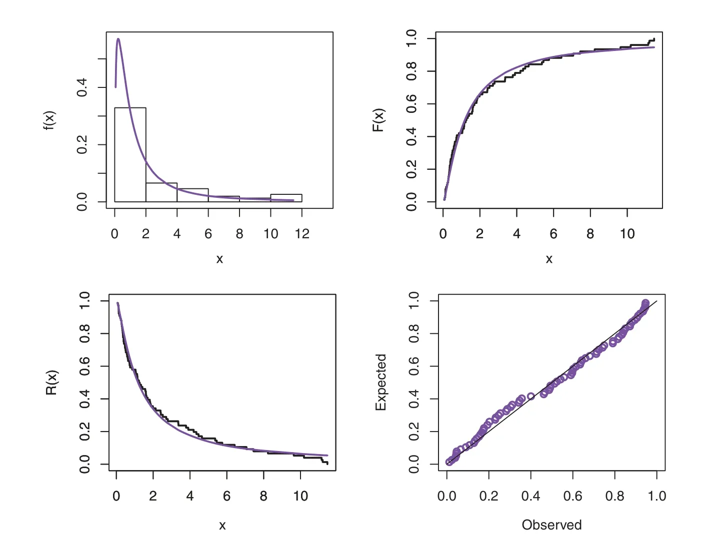
Figure 4:Plots of the fitted functions for the MAPTIW distribution and PP plot for Data 1
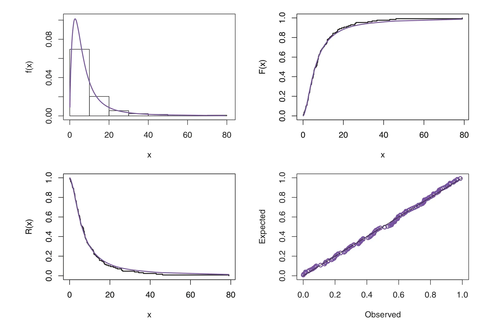
Figure 5:Plots of the fitted functions for the MAPTIW distribution and PP plot for Data 2
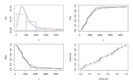
Figure 6:Plots of the fitted functions for the MAPTIW distribution and PP plot for Data 3
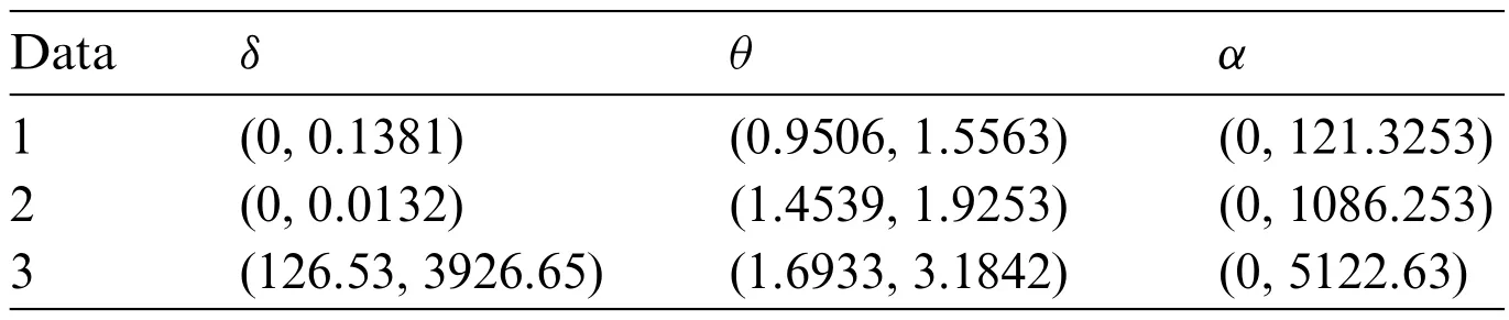
Table 8: The ACIs of the unknown parameters for Data 1,2 and 3
7 Conclusion
As a new extension of the inverse Weibull model,we introduced a new three-parameter inverse Weibull distribution.Additionally,numerous theoretical properties of the distribution were explored in order to develop a more flexible model that includes the decreasing and unimodal shape for the hazard rate function.We described the method of maximum likelihood for estimating the parameters of the suggested distribution.A simulation study is also used to investigate the asymptotic behaviour of the maximum likelihood estimators.The model’s efficiency is demonstrated using three real data sets to show its applicability in real life.The proposed distribution is a better distributional model for fitting such data sets than many of its related models,as well as several newly produced distributions,using various information measures.
Acknowledgement: The authors convey their sincere appreciation to the reviewers and the editors for making some valuable suggestions and comments.The authors extend their appreciations to Princess Nourah bint Abdulrahman University Researchers Supporting Project No.(PNURSP2022R50),Princess Nourah bint Abdulrahman University,Riyadh,Saudi Arabia.
Funding Statement: This research was funded by Princess Nourah bint Abdulrahman University Researchers Supporting Project No.(PNURSP2022R50),Princess Nourah bint Abdulrahman University,Riyadh,Saudi Arabia.
Conflicts of Interest:The authors declare that they have no conflicts of interest to report regarding the present study.
 Computer Modeling In Engineering&Sciences2023年5期
- Computer Modeling In Engineering&Sciences的其它文章
- Explicit Topology Optimization Design of Stiffened Plate Structures Based on the Moving Morphable Component(MMC)Method
- Towards a Unified Single Analysis Framework Embedded with Multiple Spatial and Time Discretized Methods for Linear Structural Dynamics
- Developments and Applications of Neutrosophic Theory in Civil Engineering Fields:A Review
- Surface Characteristics Measurement Using Computer Vision:A Review
- Recent Progress of Fabrication,Characterization,and Applications of Anodic Aluminum Oxide(AAO)Membrane:A Review
- Challenges and Limitations in Speech Recognition Technology:A Critical Review of Speech Signal Processing Algorithms,Tools and Systems