Topology Optimization for Harmonic Excitation Structures with Minimum Length Scale Control Using the Discrete Variable Method

Hongliang Liu,Peijin Wang,Yuan Liang,Kai Long and Dixiong Yang

1Key Laboratory of Liaoning Province for Composite Structural Analysis of Aerocraftand Simulation,College of Aerospace Engineering,Shenyang Aerospace University,Shenyang,110136,China

2State Key Laboratory of Structural Analysis for Industrial Equipment,Department of Engineering Mechanics,Dalian University of Technology,Dalian,116023,China

3State Key Laboratory for Alternate Electrical Power System with Renewable Energy Sources,North China Electric Power University,Beijing,102206,China

ABSTRACT Continuum topology optimization considering the vibration response is of great value in the engineering structure design.The aim of this study is to address the topological design optimization of harmonic excitation structures with minimum length scale control to facilitate structural manufacturing.A structural topology design based on discrete variables is proposed to avoid localized vibration modes,gray regions and fuzzy boundaries in harmonic excitation topology optimization.The topological design model and sensitivity formulation are derived.The requirement of minimum size control is transformed into a geometric constraint using the discrete variables.Consequently,thin bars, small holes, and sharp corners, which are not conducive to the manufacturing process, can be eliminated from the design results.The present optimization design can efficiently achieve a 0-1 topology configuration with a significantly improved resonance frequency in a wide range of excitation frequencies.Additionally,the optimal solution for harmonic excitation topology optimization is not necessarily symmetric when the load and support are symmetric,which is a distinct difference from the static optimization design.Hence,one-half of the design domain cannot be selected according to the load and support symmetry.Numerical examples are presented to demonstrate the effectiveness of the discrete variable design for excitation frequency topology optimization,and to improve the design manufacturability.

KEYWORDS Discrete variable topology optimization;harmonic excitation;minimum length scale control;geometric constraint;manufacturability

1 Introduction

Topology optimization can result in innovative structural designs via the determination of the optimal material distribution under predefined constraints without prior knowledge.In recent years, structural topology optimization has been developed rapidly and applied extensively.Various optimization methods have become effective tools for engineering structure design [1,2], such as homogenization-based method [3], density-based SIMP (solid isotropic material with penalization)method [4-6], evolutionary optimization method [7], independent continuous mapping method [8],level-set method[9,10],component-based optimization method[11],and feature-driven optimization method[12].These approaches have been extensively used to solve various structural design problems.

Because engineering structures require an increasing level of dynamic performance, topology optimization involving structural vibration characteristics is critical [13-16].Currently, topology optimization considering structural dynamic performance is garnering attention.The study includes topology optimization under harmonic excitation[17-23],topological optimization with fundamental frequency maximization [24-29], topological optimization considering high-order natural frequency maximization or frequency bandwidth optimization [30,31], and the corresponding indicators for measuring the structural vibration effect as constraints for modeling [32,33].Zargham et al.[34]provided a comprehensive review of structural dynamic topology optimization based on different optimization methods.

Structural topology optimization that considers external harmonic excitation has received considerable attention.Ma et al.[35] performed a study to minimize structural dynamic compliance under volume constraints.When the excitation frequency exceeded the first resonance frequency,the structural dynamic compliance minimization with volume constraints was investigated [36].In this case,invalid locally optimal solutions may be yielded,and static compliance constraints can be added to avoid such a phenomenon.Meanwhile,Niu et al.[19]compared different objective functions,and stress-constrained topology designs were achieved[37].Notably,the density-based method is the most widely applied method to topology design under harmonic excitation.However, the optimization results contain unavoidable gray areas (intermediate densities), particularly when considering the inertial effect of harmonic excitation.Intermediate densities may cause numerical problems in dynamic topology optimization, i.e., typically localized vibration modes [38], which need to be addressed via additional techniques [39].By merely truncating the intermediate densities, the objective function associated with the harmonic excitation may be degenerated significantly.Meanwhile, gray regions and fuzzy boundaries are not conducive to the extraction and control of geometric information from the optimization result;furthermore,they affect the structural manufacturing[40].

To improve manufacturability, topological design considering minimum length scale control is crucial.Furthermore, it is an efficient technique for addressing numerical instabilities in design optimization,such as mesh dependence and checkerboard patterns[41].Although density filtering can avoid mesh dependence and checkerboard patterns,the gray region formed at the structural boundary expands as the filtering radius increases,which implies that the minimum length scale cannot be strictly controlled.Additionally,three-field SIMP methods utilizing nonlinear projection techniques tend to yield 0-1 designs, and the minimum size may not be strictly satisfied [42,43].Based on the threefield SIMP method, a robust formulation considering corrosion and expansion operations as well as a geometric constraint method without additional finite element analysis were proposed [44,45].Meanwhile,the minimum length scale control of the topology design can be imposed using a structural skeleton[46]and an image morphology operator[47].It is worth noting that the length scale control was not applied to the topology optimization of harmonic excitation structures in previous studies.Many thin bars, small holes, and sharp corners may appear in the optimization results of harmonic excitation structures.Thus,clear and smooth topology designs with minimum length scale control are desirable for the manufacturing process.

Symmetry is an important and appealing property for structural topology optimization, as it significantly reduces the computational cost.The symmetry of optimal solutions in structural topology optimization has received significant attention [48-50].However, when the loading and support conditions are symmetric,the existence of the symmetric property in the harmonic excitation topology design problem should be verified.

In the present work, a topological design method based on discrete variables [51] is employed to resolve the topology optimization of harmonic excitation structures with length scale control.The discrete variable method is based on SAIP (sequential approximate integer programming)and CRA (canonical relaxation algorithm), which can avoid gray problems and achieve clear 0-1 solutions in topology optimization [52,53].Compared with the branch-and-bound method [54], it exhibits polynomial time complexity;thus,its computational efficiency is higher.In addition,unlike the Lagrange relaxation method, it does not require the solving of non-smooth dual optimization problems [55].Compared with the well-known evolutionary structure optimization method [56], it can manage multiple constraints via a unified mathematical programming framework,such as the size control constraints discussed herein.In this study,an optimization model is established by considering the structural dynamic compliance optimization under volume constraints, and the corresponding sensitivity formulas are derived.Furthermore, results show that the topology design solution of the harmonic excitation optimization problem may not necessarily be symmetric,even when the load and support are symmetric,which is different from the static compliance problem.

2 Discrete Variable Topology Optimization under Harmonic Excitation

2.1 Objective Function of Design Optimization

The motion equation of the harmonic excitation problem can be expressed as[19]

whereKandMdenote stiffness and mass matrices,respectively;Cdenotes the damping matrix;andrepresent acceleration and velocity, respectively;Fis the prescribed amplitude;ωis the excitation frequency.By settingu=Ueiωt,whereUdenotes the displacement amplitude,the governing equation can be rewritten as

Subsequently,the following equation can be obtained

The structural dynamic compliance is defined as

Here,c=cR+icS,wherecRandcSare the real and imaginary components ofc,respectively.When the excitation frequencyωis zero,the dynamic compliance can be degenerated into static compliance.

In this study, the square of the dynamic compliance is employed as the objective function for topology optimization[21],which can be expressed as

2.2 Optimization Formulation of Discrete Variable Topology Design

In this study, minimization of the square of structural dynamic compliance with the volume constraint is considered,and the corresponding optimization formulation based on discrete variables can be expressed as follows:

whereρ= [ρ1,ρ2,...,ρN]is a set of design variables;Nis the number of elements;veis the elemental volume;Vdenotes the predefined volume fraction.

The design variable in Eq.(6)is maintained as either 0 or 1,which allows material interpolation to be selected more flexibly because the intermediate densities need not necessarily be penalized.In fact,the material interpolation scheme of the present design is only for performing an efficient sensitivity analysis,which does not require an additional structural analysis.The global matricesKandMcan be expressed as follows:

whereKeandMeare elemental stiffness and mass matrices,respectively;Eminis an extremely low value to avoid singularity in the computation process.As demonstrated in the numerical examples,when the penalty coefficients are set asp=1,q=1 orp=3,q=1,0-1 topology designs are achievable.

3 Discrete Variable Topology Optimization Based on SAIP

3.1 Subproblem of SAIP

The discrete variable optimization method transfers the large-scale implicit nonlinear integer programming of Eq.(6) into the following explicit sequential approximate integer programming subproblem(shown in Eq.(8))based on the sensitivity of the discrete variable:

Here,beis the sensitivity of the discrete variable,which is defined as

whereρekdenotes the design variable of the current iteration.The discrete requirement ofρe∈{0,1}is equivalently transferred to the equality constraintρe(ρe-1)=0.The equality and volume constraints are introduced into the Lagrange function,which is high-order differentiable and defined in Euclidean space.Subsequently,a smooth and differentiable dual function is constructed using first-order stability conditions[51].Furthermore,an efficient CRA is employed to solve Eq.(8).

3.2 Sensitivity Analysis

Using the discrete variable sensitivity expressed in Eq.(9)incurs a significant amount of computational cost.To obtain the discrete variable sensitivity efficiently,the derivative of the objective function pertaining to the design variable can be expressed as

where the equivalent stiffness matrix is

The derivative ofKdassociated with the design variable can be calculated as follows:

where the derivative ofKpertaining to the design variable can be calculated in the same manner as that presented in[51],as follows:

and the derivative ofMregarding to the design variable can be calculated by

The proportional damping matrixCcan be expressed asC=αM+βK,whereαandβare the constant damping coefficients.The derivative of the damping matrix with respect to the design variable is expressed as

Whenp＞1,the sensitivity of the discrete variable is equal to that of the continuous variable.The sensitivity of the white element requires specific processing,as in Eq.(13),whenp=1[52].

4 Geometrical Constraint for Minimum Length Scale Control

The optimization result of the topology design may contain thin bars, small holes, and sharp corners; thus, a geometrical constraint is utilized for size control [53].If the length scale control of the material phase is satisfied,then it must be filled with the material(black),which is composed of a series of black disks with a specified radius.Similarly,if the length scale control of the void phase is satisfied,then the nonstructural zone must be filled with the void material(white),which is combined with a series of white-disks with a specified radius.Because the discrete variable method can achieve a 0-1 topological design,the definition of the minimum length scale above can be directly utilized to formulate a valid geometrical constraint.

4.1 Geometrical Constraint Function

The locally averaged element density within a specified radiusRis defined as

whereρjis a discrete design variable.Meanwhile,Neis a set of elementeat the specified radiusR,which is defined as

where (xe,ye) and (xj,yj) are the coordinates of the corresponding elemental center points.represents an integer rounded up to a specified radiusR.Based on Eq.(17),Neis a rectangular region.Because the finite element meshes used in this study are square meshes with unit sizel=1,the relationship between the minimum size radiusand the specified radius can be written as follows:

Because the design variable is discrete, the density at the structural boundary must change considerably such that the gradient value of the locally averaged densitycan be utilized to distinguish the interior,exterior,and boundary of the structure.The following expressions are defined for the structural internal and external indicators:

whereθ(·)is defined as

Here,the minimum size of the material and void phases can be controlled by settingd=R2.The central difference scheme is used to calculate the locally averaged densityIfρe= 1 andthen elementebelongs to the interior of a structure, andII(ρe) = 1.By contrast, ifρe=0 andthen elementebelongs to the outside of a structure,andIE(ρe)=1.

To satisfy the requirement of minimum length scale control,the local average density inside the structure is set to 1, whereas the local average density outside the structure is set to 0.Hence, the following geometrical detection function can be constructed:

However, the boundary elements are typically present in the structure.Even if the structure satisfies the size-control constraint,the value obtained using Eq.(21)cannot be completely equal to zero;furthermore,it is significantly smaller than the corresponding value of the structure that violates the minimum length scale.Therefore,the geometrical constraint function is expressed as follows:

The right-end termG*can be determined using the constraint relaxation strategy,as follows:

whereρkis the design variable of the current iteration,andρ0is the initial design.ζis an extremely small number and is set to 0.01.represents a reduction in the expected value of the geometrical constraint function in each iteration.

The nonlinear constraint in Eq.(23) can be linearized using the discrete variable sensitivity via a difference operation.The resulting integer programming problem with multiple constraints can be efficiently solved using the CRA.

The material layout and contribution terms are presented in Fig.1.ForR=4 and 8,the material contribution terms in Eq.(21) are shown in Figs.1a and 1b, respectively.As shown in the figures,slender rods,pointed hinges,small holes,and sharp corners that do not satisfy the requirement of the minimum size are identified.If the value of the geometric constraint function in Eq.(21)is reduced,then the topological details of the structure that do not satisfy minimum size control can be successfully eliminated.

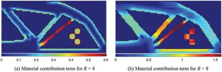
Figure 1:Material layout and material contribution term

4.2 Optimization Formulation of Minimum Length Scale Control

A relaxed linear constraint is applied to the minimum length scale control using the discrete variable sensitivity of the geometrical constraint function.Therefore, the SAIP subproblem of the topology design for harmonic excitation structures is formulated as

The CRA is employed to solve the optimization problem expressed in Eq.(24)until the variations of the adjacent objective function and constraint function are less than the specified tolerance, thus resulting in design results that fulfill the minimum length scale requirement.Accordingly,the flowchart of harmonic excitation topology optimization with minimum length scale control based on the discrete variable method is shown in Fig.2.

Figure 2:The procedure flowchart

5 Symmetry of Optimal Design under Harmonic Excitation

The optimal solution of the static problem must be symmetric when the load and support are symmetric.For frame topology optimization with the constraint of fundamental frequency, the optimal solution can be asymmetric, even when the geometry, material distribution, and structure are symmetric [48].Guo et al.[49] employed group theory to investigate the symmetry problem of structural optimization, including static compliance optimization and fundamental frequency optimization.However,the symmetry results for harmonic excitation topology optimization were not presented, and the specific reason for the asymmetric solution was not divulged.In this section, we prove that the optimal solution of the harmonic excitation problem may be asymmetrical even when the load and support are symmetric.In this regard,the three-bar truss problem,as illustrated in Fig.3,is investigated.

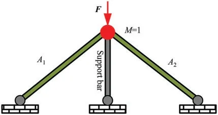
Figure 3:The three-bar truss structure

The design variables are the cross-sectional areas of the members,namelyA1andA2.The members are assumed to contribute only to the stiffness and not the mass, and a concentrated mass exists at the degree-of-freedom position with a magnitude of 1, and the Young’s modulus is unity.The corresponding stiffness and mass matrices are expressed as follows:

This model was utilized to investigate the symmetry problem of fundamental frequency optimization in[50].In this study,the model is employed to discuss the symmetry problem of structural topology optimization under harmonic excitation.The external harmonic vibration load is set as follows:

Assuming that damping is not considered tentatively, the optimization formulation for the minimum dynamic compliance with a specified amount of material can be written as

The variable is specified as a continuous variable.Owing to the absence of damping,the objective function is expressed as

Based on Eq.(27),it can be expressed as

The dynamic compliance can be written as

Subsequently,it can be transformed into the following explicit quasi-unconstrained optimization problem:

The convexity of the explicit optimization problem under various external load frequencies is analyzed herein.To facilitate the derivation, we seta=ω2.The first and second derivatives of the dynamic compliance are expressed as follows:

Next, we explain that if the second derivative of the dynamic compliance is positive under the conditiona=ω2,then the original optimization problem is convex and a symmetric optimal solution exists[50].Otherwise,the optimal solution may be asymmetrical.Based on the convexity requirement,the following nonlinear inequality equation is solved:

Eq.(33)can be described based on the following two conditions:

According to Condition I,∀A2∈[0,1],a2-3a+2≠(2A2-1)2.Thus,the range of(2A2-1)2is[0,1].Subsequently,the following can be obtained:

According to Condition II,∀A2∈[0,1],-a2+3a≤20A22-20A2+7,namely ∀A2∈[0,1],-a2+Therefore, the minimum value is obtained whenA2=0.5, and Condition II can be further derived as

Based on Eqs.(35)and(36),the following conclusions can be inferred:

(3) When 1 ≤ω2＜2,the optimization problem is not convex.Furthermore,the symmetric design(A1,A2)=(0.5,0.5)is not a locally optimal solution,and the maximum value of the dynamic compliance may be achieved(the first-order stability condition is satisfied,whereas the secondorder positive definite condition is not satisfied).

To further illustrate the conclusions above, the curves of dynamic compliance change with the design variableA2under different external load frequencies are depicted.

(a) The corresponding relationship curve for an external load frequencyω2of 0.3 is shown in Fig.4.Based on the curve, the optimization problem is a convex optimization problem, and the symmetric solution is the globally optimal solution.

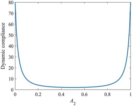
Figure 4:Relationship curve of ω2=0.3

(b) When the external load frequencyω2is 0.5,the corresponding relationship curve is as depicted in Fig.5.Because of the nonconvex nature of the optimization problem,two resonance peaks emerged when the design variables are 0.07 and 0.93.The symmetric solution is the locally optimal solution,and it remains the globally optimal solution in terms of dynamic compliance.

(c) When the external load frequencyω2is 1.1,the corresponding relationship curve is as shown in Fig.6.In this case,the symmetric design is not a locally optimal solution but achieves the maximum dynamic compliance.In this case,the globally optimal solution is(A1,A2)=(1,0)or(0,1),which is an asymmetric design.

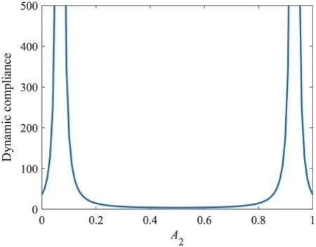
Figure 5:Relationship curve of ω2=0.5

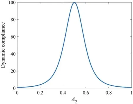
Figure 6:Relationship curve of ω2=1.1

(d) When the external load frequencyω2is 2.1,the corresponding relationship curve is as shown in Fig.7.In this case,two resonance peaks emerged.The optimization problem is nonconvex,and the symmetric solution is a locally optimal solution.

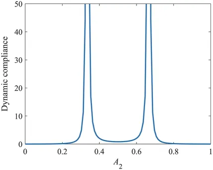
Figure 7:Relationship curve of ω2=2.1

(e) When the external load frequencyω2is equals to 3,the corresponding relationship curve is as shown in Fig.8.In this case,the optimization problem is convex,and the symmetric solution is a globally optimal solution.

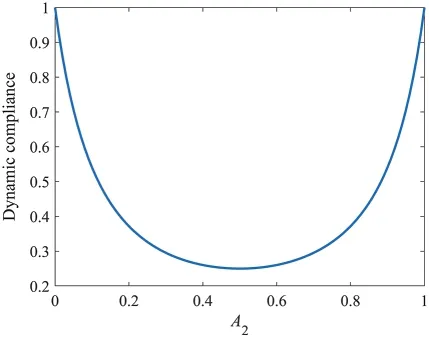
Figure 8:Relationship curve of ω2=3

In conclusion,the optimal solution of structural topology optimization under harmonic excitation may be asymmetric even when the load and support are symmetric.When the excitation frequency exceeds a certain value,the symmetric design may achieve the maximum dynamic compliance,which implies an inferior design.Therefore, unlike the static optimization problem, one-half of the design area cannot be selected for calculation based on the load and support symmetry in harmonic excitation topology optimization,which will be further discussed in the next section.

6 Numerical Examples

In this section,several numerical examples are presented to demonstrate the effectiveness of the discrete variable topology design under harmonic excitation and the geometrical constraint method.The load isF=100eiωtN.The Young’s modulus(E),Poisson’s ratio(v),and mass density of the solid material are 2.1×105MPa,0.3,and 7800 kg/m3,respectively.The proportional damping coefficients are set asα=5.24×10-1andβ=1.63×10-7.The limit of the structural volume isV= 0.5.A sensitivity filtering technique is employed to suppress checkerboard instability[42].The convergence criterion of the discrete variable design is that the relative change of dynamic compliance is less than 5×10-3.Additionally,c2andNstepare the objective function value and total iteration number of the optimized design,respectively.Grepresents the value of the geometric constraint function.

6.1 MBB Beam

First,the topological design of the MBB beam structure,as shown in Fig.9,is considered.The first resonant frequency is 1556 Hz, and the excitation frequencies are specified as 50, 500, and 1450 Hz.The structure is discretized using 240×60 bilinear finite elements with four nodes.The filtering radius is set asrmin=2.For comparison, density-based SIMP designs are presented.Notably, many gray regions and fuzzy boundaries appear in SIMP-based designs when the objective function value converges.Therefore, a constant iteration number of 300 is used for the SIMP-based designs.For an unbiased comparison, the initial designs for both the discrete variable and SIMP methods are based on full materials.The typically used initial designs in the SIMP method are the targeted volume fractions.However,the allowable excitation frequency must be decreased considerably because the first resonance frequency of the initial design is relatively low.Additionally,the initial design of the SIMP method based on a full material may incur additional numerical costs.

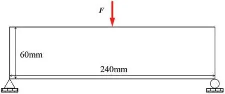
Figure 9:The MBB beam structure

The discrete variable and SIMP-based designs based onω=50 Hz are shown in Fig.10.Evidently,a 0-1 topology design is achieved when the discrete variable method is used,and the iterative number(Nstep)is 90 when the convergence criterion is used.The statistical results for the non-integer variables are shown in Table 1,where NNIVdenotes the number of non-integer variables,and“rat”denotes the ratio of the number of non-integer variables to the total number of design variables.The total number of design variables is 14400.Additionally,non-integer variables are few;thus,the rounding operation is employed to achieve an integer solution.This simple post-processing method does not significantly affect the topology design.

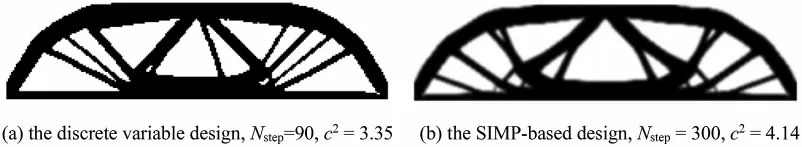
Figure 10:Topology design of the MBB beam,ω=50 Hz

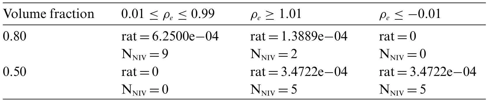
Table 1: Statistical results for the non-integer variables

By contrast, gray regions and fuzzy boundaries appear in the SIMP-based design, even though the iterative number is set to 300.The discrete variable design can avoid spurious vibration modes naturally;however,it must be deliberately addressed for SIMP-based designs,as presented in[40].In addition,the discrete variable design shown in Fig.10a is asymmetric,whereas the SIMP-based design presented in Fig.10b is symmetric.The optimal topology designs of the two methods(ω=500 Hz)are shown in Fig.11.When the excitation frequency is increased,the asymmetry of the discrete variable design is more evident,and the SIMP-based design becomes asymmetrical.Based on Figs.10 and 11,the discrete variable designs are improved by approximately 23%as compared with the SIMP-based designs.

Figure 11:Topology design of the MBB beam,ω=500 Hz

For the SIMP-based design,the measurement of the 0-1 level is expressed as[57]

whereρminis set to 0.005,andNmis the number of elemental densities exceedingρmin.WhenGR=1,the structure exhibits an all-black design,whereas whenGR=0,it exhibits an all-white design.

The optimal designs of the discrete variable method based onω=1450 Hz are shown in Fig.12.The objective value is 12.29, and the design solution is asymmetrical.The optimal topology design obtained using the symmetric boundary condition is shown in Fig.13, and the objective value is 13.86.By considering the structural symmetry, only one-half of the structure is to be calculated for topology optimization.It is evident that the objective value of the design result shown in Fig.12 is better than that presented in Fig.13.The SIMP design based onω=1450 Hz is shown in Fig.14,which is significantly different from the optimized configuration of the SAIP method shown in Fig.12.The frequency-response curves are shown in Fig.15.As shown,the first resonant frequencies of the optimized results are improved, and the asymmetrical design performs better than the symmetric design by 6%.Notably, if the initial SIMP design features intermediate densities, then structural design optimization based onω=1450 Hz cannot be implemented.However,the initial SIMP design of the full material will increase the number of computational iterations, as shown by the grayscale index in Fig.16; this implies that more iterations are required in the SIMP method to penalize the intermediate densities and achieve the 0-1 design after a fuzzy topology configuration is obtained.Based on Figs.15 and 16, when a relatively high excitation frequency is considered in the present discrete variable optimization,the design iteration is stable within 100 steps,and a faster convergence can be achieved.Furthermore, the first resonance frequency of the optimization result is improved significantly; thus, the discrete variable design can avoid resonance over a wider range of excitation frequencies.Meanwhile,the localized vibration modes can be avoided naturally.Therefore,the present discrete variable method can efficiently achieve a 0-1 optimum design with an improved resonance frequency over a wide range of excitation frequencies.

Figure 12:Discrete variable design with ω=1450 Hz,Nstep=103,c2=12.29

Figure 13:Discrete variable design utilizing the symmetric boundary condition,Nstep=97,c2=13.86,ω=1450 Hz

Figure 14:SIMP design with ω=1450 Hz,Nstep=300,c2=18.47

Figure 15:Frequency response curves

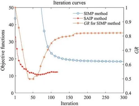
Figure 16:Iterative curves for the SAIP and the SIMP method

6.2 Clamped-Clamped Beam

A clamped-clamped beam,as shown in Fig.17,is considered in this study.Its excitation frequencyωand filtering radiusrminare 50 Hz and 2,respectively.Furthermore,it is discretized by using 240×40 bilinear finite elements with four nodes.

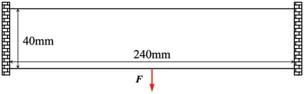
Figure 17:A clamped-clamped beam structure

In the optimal topology design of the clamped-clamped beam,as shown in Fig.18,the penalty coefficient is set asp=3,and the objective value is 2.74.The topological design based on the discrete variable method by setting the penalty coefficient top=1 is shown in Fig.19.When the penalty coefficient is set to 1, the discrete variable method can still achieve a black-and-white design with distinct topology.As shown in Fig.20,the discrete variable designs of the intermediate volume fraction are also available designs,i.e.,all the topology designs from the initial design to the predefined volume ratio(Pareto frontier)can be achieved in one optimization solution.When the excitation frequency is relatively high(approximately the first resonance frequency of the initial design)and the volume ratio is equal to 0.7, more materials are concentrated at the fixed supports, which increase the stiffness and weaken the inertia effect, as shown in Fig.21, thus reflecting the dynamic effect of topology optimization while considering harmonic excitation.

Figure 18:The discrete variable design of the clamped-clamped beam,Nstep=93,p=3,c2=2.74

Figure 19:The discrete variable design of the clamped-clamped beam,Nstep=93,p=1,c2=2.82

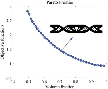
Figure 20:Pareto frontier,where the average number of finite element analysis for each Pareto frontier point is 93/35

Figure 21:The discrete variable design of the clamped-clamped beam with a relatively high excitation frequency

6.3 Cantilever Beam

In this subsection,the topological design of the cantilever beam structure,as shown in Fig.22,is discussed.Its excitation frequency isω=50 Hz,and 120×60 bilinear finite elements with four nodes are adopted.

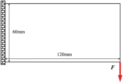
Figure 22:A cantilever beam structure

The optimal topology designs of the present discrete variable method are shown in Fig.23,where the sensitivity filtering radii are set as 2,3,4 and 5.As the filtering radius increases,finer structures are gradually filtered out,and the objective value increases.The filtering radius size can affect the optimal design configuration;additionally,it can be used to indirectly control the feature size to avoid mesh dependence.As shown in Fig.23a,the optimization result contains thin bars,small holes,and sharp corners when the filter radius is small,whereas the optimization result still contains sharp corners when the filter radius is relatively large,as shown in Fig.23d.Thus,a geometrical constraint for size control is employed,where the sensitivity filtering radius and specified radiusRare set to 2 and 6,respectively.The optimal design is shown in the third column of the first row of Table 2;it can eliminate thin bars,small holes,and sharp corners,thus improving the manufacturability of the structural design.

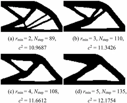
Figure 23:The discrete variable designs of the cantilever beam

Subsequently, two different finite element meshes (120×60 and 180×90) are considered.The corresponding filter radii are 2 and 3,and the radiiRof the size control are set to 6 and 9,respectively.The topology design results are presented in Table 2.For the two mesh refinements, the ratio of the filter radiusrminto the number of meshes is the same, namely 2/120=3/180.The ratio of the specified control radiusRto the number of meshes is the same as well,i.e.,6/120=9/180.This implies that the mesh-dependent designs are further optimized into mesh-independent designs that fulfill the requirement of the minimum length scale.The post-smoothing design is shown in Table 2,which is able to get the nodal density based on the elemental density,and the level set function is obtained via linear interpolation within the element based on the nodal density.The threshold of the level set is determined via dichotomy to ensure that the volume of the level set function (greater than zero) is equal to the volume constraint.Because discrete variable designs feature a 0-1 topology configuration and clear boundaries,post-smoothing will not significantly affect the objective function.Furthermore,the loss of the objective value for the smooth design is less significant when additional size control is applied.Thus,the smooth designs in Table 2 that satisfy the minimum size requirements are more convenient for the manufacturing.For example,the design can be manufactured via a machining technique where the minimum length scale is strictly restricted by the size of the machining drill[40].

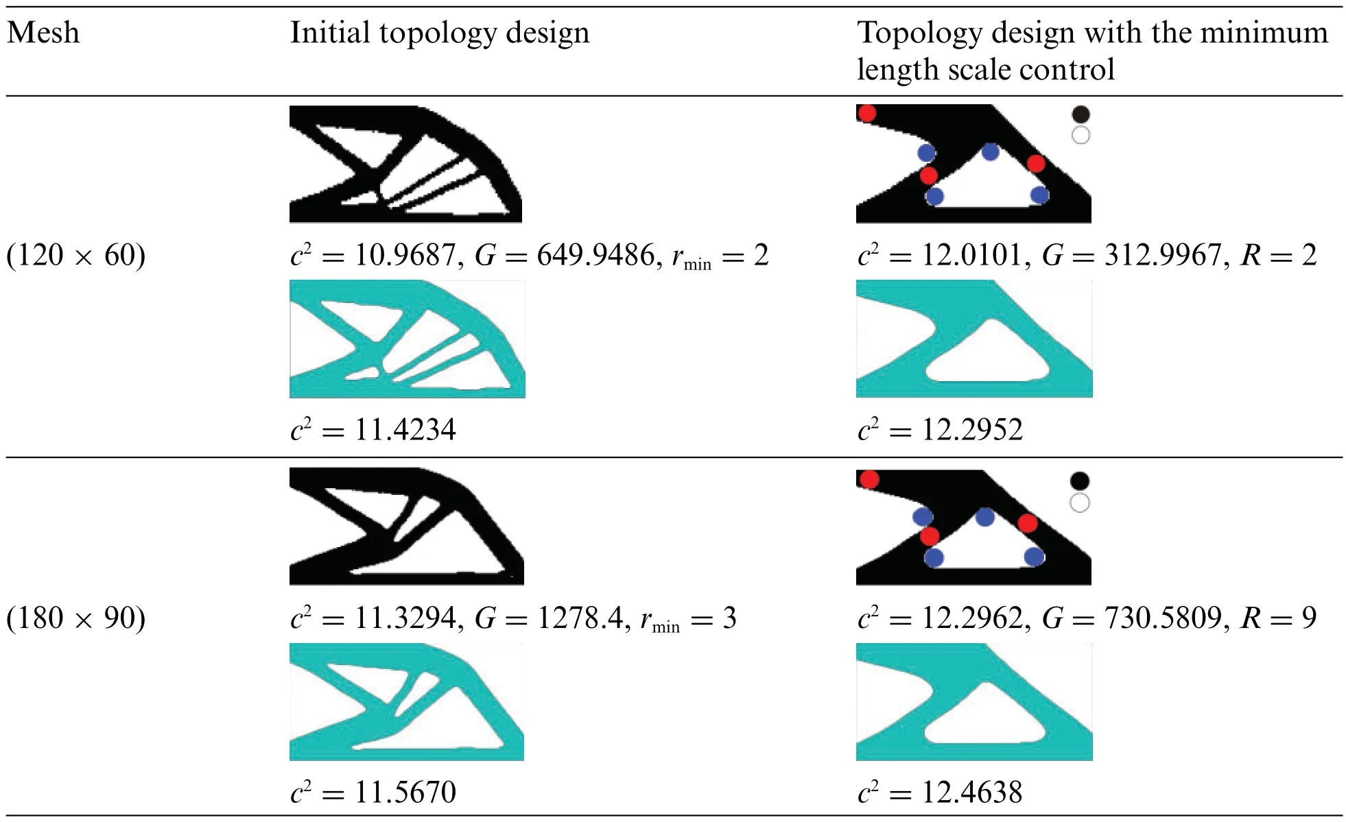
Table 2: Topology designs achieved by two different finite element meshes

7 Conclusions

In this study, the discrete variable design method is employed to perform topology design optimization under harmonic excitation.To satisfy the size control constraints in the manufacturing process, minimum length scale control is transformed into geometrical constraints and solved efficiently using the optimization framework presented herein.Subsequently, the topological design model and sensitivity formulation are derived.Compared with the solution of the classical statics problem, the optimal solution of the harmonic excitation structure is not necessarily symmetric when the load and support are symmetric.Thus, one-half of the design domain cannot be selected based on the load and support symmetry.The discrete variable method can efficiently achieve a 0-1 topology design with an improved resonance frequency over a wide range of excitation frequencies.Using the geometrical constraint for the minimum length scale control,the mesh dependence of the topology design optimization is effectively addressed, and thin bars, small holes, and sharp corners are eliminated,which improves the manufacturability of the structural design.

The geometrical constraint for the minimum length scale control only requires a calculation of the average density and average density gradient within a specified size range to be applied to the complex structure.For complex meshes, Helmholtz filtering can be utilized to efficiently calculate the local average density by solving partial differential equations, and the technique proposed by Crispo et al.[58]can be used to calculate spatial gradients.Studies will be performed in the future to identify a new method to address the minimum length scale control of engineering structure designs with complex meshes.Furthermore,the sampling points in the frequency range yield numerous finite element equations of state with different coefficients, which incur high computational costs.This issue shall be addressed in future studies.The results of this study can provide a basis for structural optimization under harmonic excitation in the frequency range, since the potential of the present algorithm for solving dynamic optimization problems is confirmed.

Funding Statement:This work was supported by the National Natural Science Foundation of China(12002218 and 12032008)and the Youth Foundation of Education Department of Liaoning Province(Grant No.JYT19034).

Conflicts of Interest:The authors declare that they have no conflicts of interest to report regarding the present study.