The Fractional Investigation of Some Nonlinear Partial Differential Equations by Using an Efficient Procedure

Fairouz Tchier,Hassan Khan,Shahbaz Khan,Poom Kumam and Ioannis Dassios

1Mathematics Department,King Saudi University,Riyadh,145111,Saudi Arabia

2Department of Mathematics,Abdul Wali Khan University,Mardan,23200,Pakistan

3Department of Mathematics,Near East University,Nicosia,99138,Turkey

4Theoretical and Computational Science(TaCS)Center Department of Mathematics,Faculty of Science,King Mongkuts University of Technology Thonburi(KMUTT),Bangkok,10140,Thailand

5Department of Medical Research,China Medical University Hospital,China Medical University,Taichung,40402,Taiwan

6AMPSAS,University College Dublin,Dublin,A94 XF34,Ireland

ABSTRACT The nonlinearity in many problems occurs because of the complexity of the given physical phenomena.The present paper investigates the non-linear fractional partial differential equations’solutions using the Caputo operator with Laplace residual power series method.It is found that the present technique has a direct and simple implementation to solve the targeted problems.The comparison of the obtained solutions has been done with actual solutions to the problems.The fractional-order solutions are presented and considered to be the focal point of this research article.The results of the proposed technique are highly accurate and provide useful information about the actual dynamics of each problem.Because of the simple implementation,the present technique can be extended to solve other important fractional order problems.

KEYWORDS Fractional calculus;laplace transform;laplace residual power series method;fractional partial differential equation;power series;fractional power series

1 Introduction

The integral and derivative of fractional order are considered to be common topics of fractional calculus (FC) due to their numerous applications in applied sciences.This topic has gained much popularity among researchers because of its popularity and significance while modelling various procedures in nature.For example,these problems are increasingly being applied to equations in fluid flow, diffusion, polymer physics, electric network rheology, relaxation, reaction-diffusion, diffusive transport akin to diffusion, turbulence, anomalous diffusion, porous structures, and dynamical processes in complex systems,as well as a variety of other physical phenomena[1,2].In the last few decades,the early theory and development regarding fractional derivatives and fractional differential equations(FPDEs)have been observed rapidly.The subject is further explained and extended by the authors, such as Abbas et al.[3], Hilfer [4], Kilbas et al.[5], and Legnani et al.[6].The systematic understanding of FC like uniqueness and existence and theoretic issues related to FPDEs are the core themes of their work.Other concepts of FC can be read in the papers of Hernández et al.[7]where the recent advances in the theory of FPDEs are presented.Magin et al.[8]and Mainardi[9]looked into FC’s applications in interdisciplinary fields like image processing and control theory.

It is very rare to calculate the exact solution of non-linear FPDEs in the literature.Using linearization, successive, or perturbation methods, only approximate solutions can be obtained.Iterative Laplace transform method[10],Adomian decomposition method[11],Homotopy analysis method [12], operational matrix method [13], fractional differential transform method [14], Fourier transform technique[15],operational calculus method[16],Variational iteration method[17],Sumudu transform method[18],multistep generalised differential transform method[19],iterative reproducing kernel method[20],Homotopy perturbation method[21],and Numerical multistep method[22].

In many cases,analytical or exact solutions are very difficult to investigate.Therefore,mathematicians have tried to develop and use several numerical techniques with fractional derivative and integral operators [23-25].In this connection, in 2017, Li et al.presented three efficient techniques, namely the finite difference method, the Galerkin finite element method, and the spectral method, for the solutions of some FPDEs[26].Atangana et al.used the fundamental theorem of fractional calculus along with the Lagrange interpolation polynomial and investigated the solution of the Keller-Segel model[27]in 2018.In 2020,the shifted Chebyshev polynomials with some assumptions were used to find the solutions of some FPDEs with variable coefficients[28].Similarly,in 2020,the finite difference method and operational matrix method were used to determine the solution of Riez-space FPDEs[29].

Without linearization,perturbation,and discretization,the residual power series method(RPSM)is an effective and uncomplicated technique for constructing a power series(PS)solution for FPDEs.Unlike the traditional PS method,the RPS method does not require a recursion relation or comparison of the coefficients of the related terms.A series of algebraic expressions are obtained to calculate the PS coefficients.The methodology’s main advantage is that it relies on simpler and more accurate derivation as compared to other techniques that are based on integration.This method is a different way of solving FPDEs in theory [30].The Laplace residual power series method (LRPSM) [31] is a combination of the Laplace transform (LT) and the RPSM.In the procedure of LRPSM, the first Laplace transformation is used to simplify the targeted problem into new algebraic equations.The RPSM is then implemented to obtain the series solution.In the end,the inverse Laplace transform is applied to attain the required solution.The LRPSM required less calculation with less time and more accuracy.

In this article, the LRPSM is used to solve the time and space FPDEs.The aim of the study is to use LRPSM with space-time fractional derivatives of the form to obtain numerical solutions to nonlinear fractional partial differential equations.

whereu(ζ,t)is assumed to be a spatial function that vanishes accordingly forζ ＜0 andt ＜0,and are parameters describing the order of the fractional derivatives ofζandt,respectively.When dealing with fractional derivatives,Caputo sense[32]is applied.

The generalized LRPSM procedure is presented and then LRPSM algorithm is applied to solve few numerical problems.The results and the accuracy of the suggested technique is shown by tables and graphs.The graphical representation is done and the obtained solutions are vary closed to the actual solutions of each target problem.The fractional order LRPSM solutions provide the analysis of some useful dynamics of the given FPDE’s.The tables have shown that LRPSM has the higher degree accuracy.LRPSM is comparatively a very simple and direct procedure to evaluate the solutions of nonlinear FPDEs and their systems.The proposed required fewer calculations to compute the non-linear terms in each problem.

The article layout as follows.The fundamental concepts regarding FC are described in Section 2,the basic methodology is discussed in Section 3,the effectiveness of LRPSM is confirmed by some test models in Section 4,results and discussion are in Section 5 and the conclusion is given in Section 6.

2 Basic Definitions

2.1 Definition

The Caputo’s derivative off(t)is given as[33]

2.2 Definition

LetT ＞0,g∈H1(0,T),andζ∈(0,1);then theζthCaputo-Fabrizio derivative offis given as

wherem=,andM(ζ)is a normalizing function depending onζ,such thatM(o)=M(1)=1.

In[34],Losada and Nieto provided an explicit formula forM(ζ)as.In this case,the Caputo-Fabrizio derivative Eq.(2)is reduced to

2.3 Definition

Letf∈H1(a,b),a ＜bandζ∈[0,1].The Caputo Atangana-Baleanu fractional derivative[35,36]offof orderζis defined by

whereEζ(t) is Mittag-Leffler function defined [4,7]andM(ζ) is a normalizing function.

2.4 Theorem

(Fractional Taylor’s formula[37])Let us assume thatf(t)has a FPS representation att=0 of the form

Iff(t) ∈C[0,R]and) ∈C(0,R)forn= 0,1,2,...,then the coefficientsbnin the Eq.(1)can be written as

whereDntξ=Dξt.Dξt···Dξt(n-times).

2.5 Theorem

Suppose thatf0has a fractional power series expression of the form att=t0

IfDθt ξu(ζ,t),θ=0,1,...are continuousI×(t0,t0+R),then the coefficientfθ(ζ)can be defined as

2.6 Definition

A PS representation of the form

where 0 ≤n-1＜ξ≤n,τ≤τ0is known as fractional power series(FPS) aboutτ0, wherePnthe coefficient of the series.Ifτ0= 0 then FPS will be reduced to a fractional Maclaurin series at that point.

2.7 Definition

The extension form of PS is

is called multi FPS aboutt=t0,wherefn(ζ)are the coefficients of multi FPS.

2.8 Theorem

Consider thatu(ζ,t)has a many FPS representation att=t0of the form

IfDjξu(ζ,t),j=0,1,2,...are continuous onI×(t0,t0+R),then

3 The Methodology of LRPSM

Here,we will go through the procedure that LRPSM takes to solve time and space FPDEs.

with initial condition(IC)

We apply the LT to Eq.(9),i.e.,

whereU(ζ,s)=Lt[u(ζ,t)].

We write the Eq.(12)as the following expansion:

Thekth-truncated series of Eq.(13)takes the form

As stated in[31],the definition of Laplace Residual(LR)function to Eq.(12)is

and thekth-LR function of Eq.(15)is

here are some properties arise in the RPSM[31],to point out some facts:

•LtResk(ζ,s)=0 and limk→∞=LtRes(ζ,s)for eachs ＞0.

• lims→∞sLtRes(ζ,s)=0 ⇒lims→∞sLtResk(ζ,s)=0.

• limx→∞skξ+1LtRes(ζ,s)=lims→∞skξ+1LtResk(ζ,s)=0,0＜ξ≤1,k=1,2,3,...

Therefore,to determine the coefficient functionsfn(ζ),we solve recursively,the following system

We apply the inverse LT toUk(ζ,s),to obtain thekth-approximate solutionuk(ζ,t).

4 Numerical Problems

4.1 Problem 1

Consider the time and space FPDE[38]

with IC

We apply the LT to Eq.(16)and using of Eq.(17),i.e.,

Thekth-truncated series of Eq.(19)takes the form

and thekthLR function of Eq.(19)

Now, to determinefk(ζ),k= 1,2,3,..., by putting thekth-truncated series Eq.(20) into thekthLaplace Residual function Eq.(21),multiply the resulting equation byskξ+1,and then recursively solve the relation lims→∞[skξ+1Resk(ζ,s)]=0,k=1,2,3,...forfk(ζ).The first few elements of the sequences

Putting the values offn(ζ),(n≥1)in Eq.(4),we have

Applying inverse LT to Eq.(23),we get

puttingξ=ρ=1 in Eq.(24),we get the solution in closed form

4.2 Problem 2

Consider the time and space FPDE[38]

Finally the last day of school arrived and the elf was free to go. As for homework, there was no more, so he quietly and slyly slipped out the back door.

with initial condition

exact solution of Eq.(26)atξ=ρ=1 is

We apply the LT to Eq.(26)and making use of Eq.(27)i.e.,

Thekth-truncated series of Eq.(29)takes the form

and thekthLR function of Eq.(29)

Now,to determinefk(ζ),k=1,2,3,...,we substitute thekth-truncated series Eq.(30)into thekthLaplace Residual function Eq.(31),multiply the resulting equation byskξ+1,and then recursively solve the relation lims→∞[skξ+1Resk(ζ,s)] = 0,k= 1,2,3,...forfk(ζ).First few elements of the sequences

Putting the values offn(ζ),(n≥1)in Eq.(30),we have

Applying inverse LT to Eq.(33),we get

Puttingξ=ρ=1 in Eq.(34),we get the solution in closed form

4.3 Problem 3

Consider the time and space FPDE[38]

with IC

exact solution of Eq.(36)atξ=ρ=1 is

We apply the LT to Eq.(36)and making use of Eq.(37),i.e.,

Thekth-truncated series of Eq.(39)takes the form

and thekthLaplace Residual function of Eq.(39)

Now,to determinefk(ζ),k=1,2,3,...,we substitute thekth-truncated series Eq.(40)into thekthLR function Eq.(41),multiply the resulting equation byskξ+1,and then solve recursively the relation lims→∞[skξ+1Resk(ζ,s)] = 0,k= 1,2,...forfk(ζ).The first few elements of the sequencesfk(ζ) as follows:

Putting the values offn(ζ),(n≥1)in Eq.(40),we have

Applying inverse LT,we get

puttingξ=ρ=1,the solution in closed form is

5 Results and Discussion

Figs.1 and 2 present the 2D and 3D plots of the Exact and LRPSM solutions at different fractional order’s of Example 4.1.The exact and LRPSM solutions in integer order are in closed contact with each other.It is observed that the fractional solutions are convergent towards integer order solution,which confirmed the validity of the suggested method for fractional order problems.Tables 1,2 and 4 discuss the absolute error associated with LRPSM solution at different time level and spaces of Examples 4.1, 4.2 and 4.3.It is noted that as the fractional-orders approach to integer order, the method’s accuracy is increased.This phenomenon supports the applicability of LRPSM to fractionalorder solutions.The tables have confirmed the convergence of the fractional solutions towards integer order solutions.In Table 3,the LRPSM solutions are compared with ADM solutions.The solutions comparison has shown that LRPSM has greater accuracy as compared to ADM.Figs.3 and 4 show the 2D and 3D plots of exact and LRPSM solutions at different fractional orders of Example 4.2.Also,Figs.5 and 6 provide the 2D and 3D plots of the exact and LRPSM fractional solutions of Example 4.3, respectively.The overall discussion of the graphs and tables reveals that the LRPSM solutions are more accurate and effective.The overall comparison of LRPSM and exact solutions provided the sufficient and closed relation with each other.The convergence of fractional solutions towards the integer order solution is observed.Table 5 represents the list nomenclatures that have been used to abbreviate various kinds of important names in the paper.

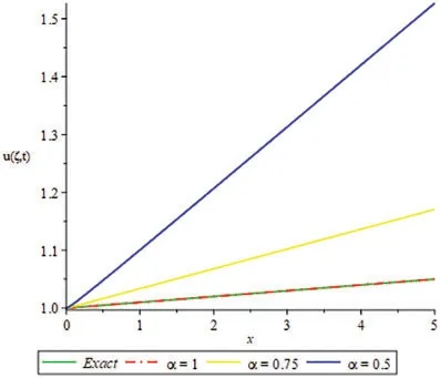
Figure 1:2D plots for exact and LRPSM solution of Example 4.1 for different values of ξ

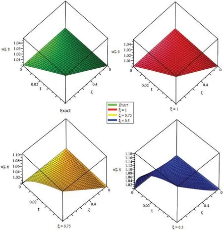
Figure 2:3D plots exact and LRPSM solution of Example 4.1 for different values of ξ

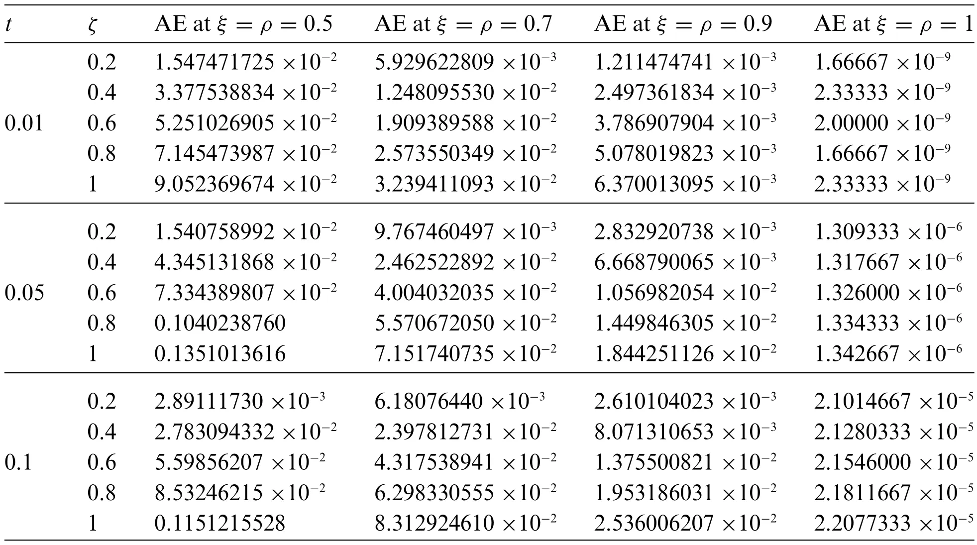
Table 1: Absolute Error(AE)for different times and spaces of Example 4.1

Table 2: Absolute Error(AE)for different times and spaces of Example 4.2

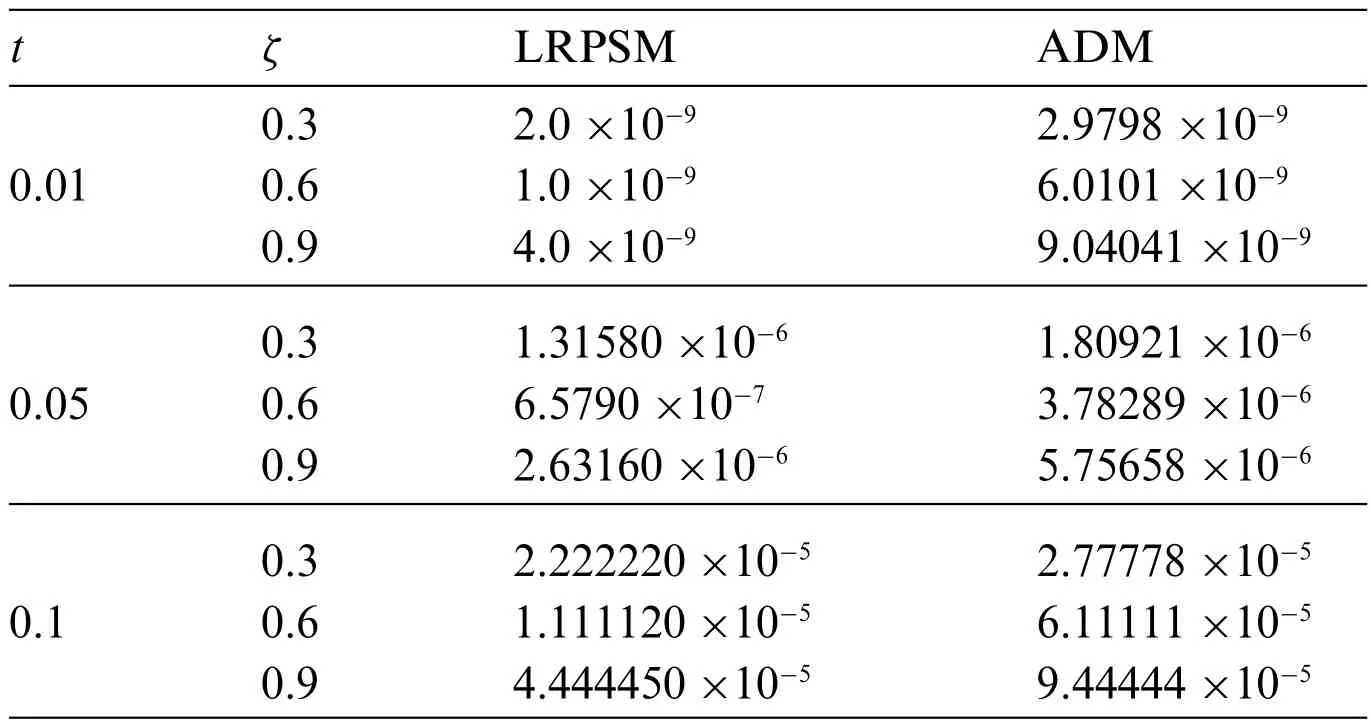
Table 3: Absolute Error(AE)comparison of LRPSM and ADM[39]for Example 4.2

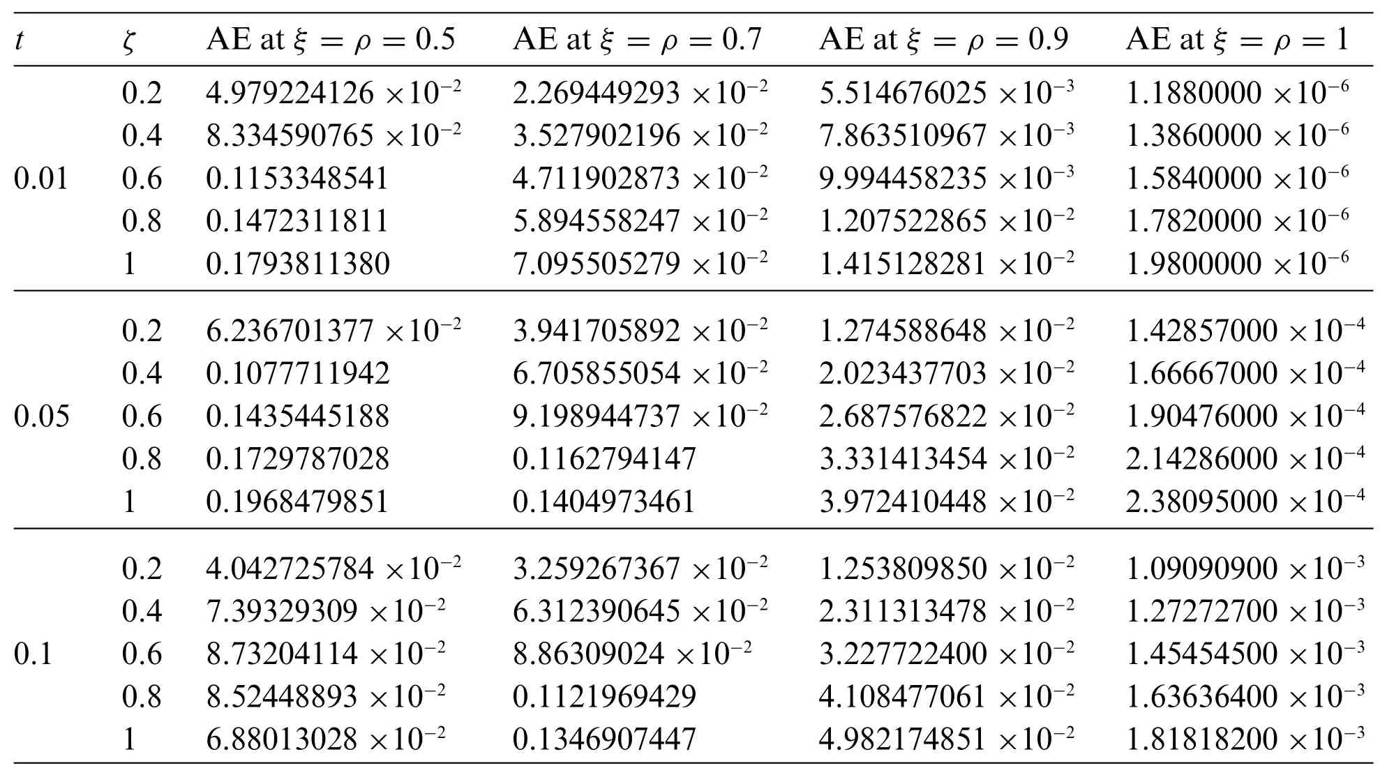
Table 4: Absolute Error(AE)for different times and spaces of Example 4.3

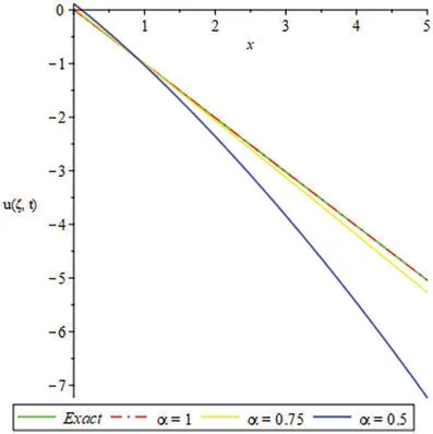
Figure 3:2D plots for exact and LRPSM solution of Example 4.2 for different values of ξ

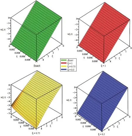
Figure 4:3D plots for exact and LRPSM solution of Example 4.2 for different values of ξ

Figure 5:2D plots for exact and LRPSM solution of Example 4.3 for different values of ξ

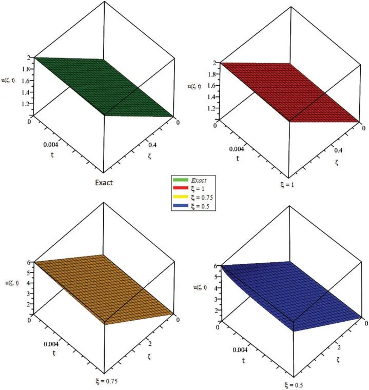
Figure 6:3D plots for exact and LRPSM solution of Example 4.3 for different values of ξ

Table 5: Nomenclature

6 Conclusion

The present article is related to the approximate analytical solutions of some nonlinear fractional partial differential equations using the Laplace residual power series method.The fractional derivatives in each targeted problem are represented by the Caputo operator.First, the proposed scheme is discussed for the general nonlinear problem and the few nonlinear problems related to nonlinear fractional partial differential equations are solved by using the proposed method.The obtained results are compared with the exact solution of each problem.The fractional order solutions are analyzed by using the suggested method successfully.It is observed that the present technique is the most suitable tool for the solutions of nonlinear fractional partial differential equations and possesses a higher degree of accuracy.In conclusion,this new hybrid technique is straightforward to solve the nonlinear fractional problems and can be used effectively in other branches of applied sciences.

Authors Contribution:Fairouz Tchier (Investigation, Draft Writing), Hassan Khan (Supervision),Shahbaz Khan (Methodology, Investigation) Poom Kumam (Funding, Draft Writing), Ioannis Dassios(Draft Writing).

Availability of Data and Material:Not applicable.

Funding Statement:Researchers Supporting Project No.(RSP-2021/401), King Saud University,Riyadh,Saudi Arabia.

Conflicts of Interest:The authors declare that they have no conflicts of interest to report regarding the present study.