On the Approximation of Fractal-Fractional Differential Equations Using Numerical Inverse Laplace Transform Methods

Kamran,Siraj Ahmad,Kamal Shah,Thabet Abdeljawadand Bahaaeldin Abdalla

1Department of Mathematics,Islamia College Peshawar,Khyber Pakhtoon Khwa,Peshawar,25120,Pakistan

2Department of Mathematics and Sciences,Prince Sultan University,P.O.Box 66833,Riyadh,11586,Saudi Arabia

3Department of Mathematics,University of Malakand,Chakdara Dir(L),Khyber Pakhtunkhwa,18000,Pakistan

4Department of Medical Research,China Medical University,Taichung,40402,Taiwan

ABSTRACT Laplace transform is one of the powerful tools for solving differential equations in engineering and other science subjects.Using the Laplace transform for solving differential equations,however,sometimes leads to solutions in the Laplace domain that are not readily invertible to the real domain by analytical means.Thus,we need numerical inversion methods to convert the obtained solution from Laplace domain to a real domain.In this paper,we propose a numerical scheme based on Laplace transform and numerical inverse Laplace transform for the approximate solution of fractal-fractional differential equations with order α,β.Our proposed numerical scheme is based on three main steps.First, we convert the given fractal-fractional differential equation to fractional-differential equation in Riemann-Liouville sense,and then into Caputo sense.Secondly,we transform the fractional differential equation in Caputo sense to an equivalent equation in Laplace space.Then the solution of the transformed equation is obtained in Laplace domain.Finally,the solution is converted into the real domain using numerical inversion of Laplace transform.Three inversion methods are evaluated in this paper,and their convergence is also discussed.Three test problems are used to validate the inversion methods.We demonstrate our results with the help of tables and figures.The obtained results show that Euler’s and Talbot’s methods performed better than Stehfest’s method.

KEYWORDS Fractal-fractional differential equation;power law kernel;exponential decay kernel;Mittag-Leffler kernel;Laplace transform;Euler’s method;Talbot’s method;Stehfest’s method

1 Introduction

Fractional calculus(FC)is the generalization of classical calculus in which we study the differential and integral operators of non integer order.FC can explain numerous real world phenomena with a better memory effect.Initially,fractional calculus was treated as an abstract mathematical idea with almost no application.But within the last few decades,a significant development has been observed in the fields of FC,such as Geo-Hydrology,chaotic processes[1,2],wave propagation,rheology,finance system[3],groundwater flow,and fluid mechanics[4,5],fractional-order dynamical systems in control theory[6],fractional order controller[7],fractional Brownian motion[8],generalized Mittag-Leffler function [9] etc.Until now, various operators of arbitrary order have been introduced in which the two most commonly used with singular kernels are Riemann-Liouville (RL) and Caputo.Similarly,the two famous fractional derivatives with non singular kernels which have been used in literature are the Caputo-Fabrizio (CF) and Atangana-Baleanu (AB) [1,10].Applications of these fractional derivatives with non singular kernels have been investigated by many researchers in various fields of science and engineering.Some of the reported work is discussed here.For instance,Wang et al.[11]studied fractional Fredholm integro differential equation with AB derivative.Liu et al.[12]investigated Riccati differential equation with AB derivative.Qiang et al.[13]studied Volterra integro differential equation with AB derivative.Gorenflo et al.[14]derived some results for Mittag-Leffler function and related applications.Yavuz et al.[15]investigated a fractional predator-prey model.Sulaiman et al.[16]established some numerical results for fractional coupled viscous Burger’s equation involving Mittag-Leffler kernel.

In literature,numerous methods have been proposed for the analytical and numerical solutions of problems from FC,such as the sinc-collocation method[17],Taylor collocation method[18],Adomian decomposition method[19],variation iteration method[20],RBFs method[21,22],operation matrix method[5],finite difference method[23],etc.

Recently,in[1],the author developed a new idea of fractal-fractional derivative.Fractal-fractional derivative is very suitable in many situations in dealing with real world complex phenomena.This operator has two orders,one is the fractional order and the second is fractal dimension.As compared to other fractional order operators,fractal-fractional derivative is a powerful tool to describe the complex geometry more precisely and efficiently.Usually for the description of irregular and complex geometry fractal-fractional derivative has been used as a powerful tool.The said irregular or complex geometry could not be described by the Caputo fractional derivatives[24,25].Fractal-fractional operators have not yet been studied extensively.However, few but valuable research articles are available related to the study of fractal fractional differential operators.For instance, authors [26] have developed a numerical method for the numerical solutions of differential equations of fractal-fractional order.In [27], authors have investigated the advection dispersion model.Atangana et al.[25] have derived the exact solution of some important fractal-fractional differential equations.They have also studied the numerical solution for nonlinear cases.Owolabi et al.[28] have developed numerical methods for fractal-fractional Scnakenberg reaction diffusion system.The authors in [5] have proposed an efficient operation matrix method for solving fractal-fractional differential equations.Other valuable work on fractal-fractional differential operators can be found in[29-31]and references therein.But most of these methods are based on the finite difference method for temporal discretization, and they encounter an increase of computing cost with advancing time and thus these methods have low efficiency in the simulation of the long time history of fractional differential equations.

In order to overcome the drawback of the finite difference method for temporal discretization,in this work,we propose a method based on Laplace transform(LT)and numerical inverse Laplace transform (NILT) method.The main idea of the proposed work is to use the LT to reduce the time dependent problem in Caputo sense to an equivalent time independent problem and then solve it in the LT space.Further,a solution of the considered original problem is obtained using NILT.The purpose of using the LT and NILT instead of step-by-step finite difference method for temporal discretization is to avoid the calculation of costly convolution integral in fractal-fractional derivative approximation,and avoid the time stepping technique and the severe stability restrictions in time.In this article, we have utilized three NILT methods:the Talbot’s method,the Euler’s method,and the Stehfest’s method.

The rest of the paper is organized as: in Section 1, some important definitions are given.In Section 2,the methodology of the proposed numerical scheme is described.In Section 3,the numerical examples are given.

1.1 Preliminaries

This section is devoted to some basic definitions from fractional calculus.

Definition 1.1.IfG(t)is continuous on(a,b),andG(t)is fractal-differentiable in(a,b)with orderβ,then the fractal-fractional derivative ofG(t)of orderαin RL sense is defined in[25]as

1.with power law kernel

where

2.With exponential decay kernel

3.With generalized Mittag-Leffler(ML)kernel

where

Definition 1.2.LetG(t)be piecewise continuous function defined fort ＞0.The LT ofG(t)is defined in[25]as

The three famous derivatives Caputo,CF and AB satisfy the following relations[25]:

The LT of these derivatives is given as

and

2 Proposed Method

In this section,we propose our numerical method for the approximation of the solution fractalfractional differential equations with different kernels.

2.1 Power Law Kernel

A power law is a functional relationship between two quantities, where a relative change in one quantity results in a proportional relative change in the other quantity.Power law kernels have significant applications in mathematical modeling of various real world problems.For instance,those problems are related to machines learning,where power law kernels play central role in modeling the process.Furthermore,positive definite kernels are considered as a measure of similarity between points in the kernel based machine learning procedure.Also,theoretic quantities and information based on kernels are usually used in image processing and text mining.The most significant use of power law kernels can be found in the probability distribution theory.Besides, from the mentioned fields, the important applications of the said kernels can be studied in mathematical modeling of various process of cosmology,physics and astronomy as well as in biology.Here,we consider a differential equation with power law kernel of the form[25]

which implies

then

then

then,we get

Using the relation between the Caputo and RL derivatives,(16)can be written as

Now we take LT of both side of given equation as

which implies

where

and

Simplifying,we get

Now the inverse LT of(18)gives

2.2 Exponential Decay Kernel

We consider a differential equation with exponential decay kernel[25]as

which implies

then

then

then,we get

Using the relation between the CF and RL derivatives,(24)can be written as

Now we take LT of both side of given equation

which implies

where

simplifying,we get

Now the inverse LT of(26)gives

2.3 Generalized Mittag-Leffler(ML)Kernel

We consider a differential equation with generalized ML kernel of the form[25]

which implies

then

then

then,we get

Using the relation between the AB and RL derivatives,(32)can be written as

Now we take LT of both sides of given equation

which implies

where

Simplifying,we get

Now the inverse LT of(34)gives

Now we need to approximate the inverse LT in (19), (27), and (35) numerically.In this work,we have utilized three different approaches for this purpose which are(i)Talbot’s method(ii)Euler’s method(iii)Stehfest’s method.The flowchart of the proposed numerical scheme is shown in Fig.1.

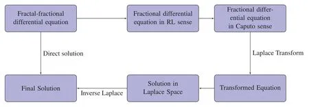
Figure 1:The flowchart of the proposed numerical scheme

2.4 Talbot’s Method(TM)

Using Talbot’s method,the solution of the given problem is obtained as

whereρ0is the converging abscissa andCis a suitably chosen line which connectsρ-ι∞andρ+ι∞,which means that all the singularities of the functionG(z)lie to the left ofC.Its very difficult to approximate the integral defined in(36)due to the highly oscillatory exponential factoreztand the slow decaying transformG(z).Talbot has suggested in his article[32]that this issue can be resolved using the contour deformation.Furthermore,he suggested that the deformation be done in such a way that real part of the contour starts and ends in the left complex plane inclosing all the singularities of the transform ˆG(z).On such contours,the integrand decays rapidly owing to the exponential factor,which makes the integral(36)suitable for approximation using the trapezoidal rule or mid point[32,33].In this work,we consider a contour of the form[33]:

whereRez(±π)=-inf,andz(θ)is given as

whereμ,ν,γare to be chosen by the user,using(38)in(36),we have

We approximate the latter integral by the N-panel midpoint rule spacing,which yields

2.4.1 Convergence of Talbot’s Method

In the approximation of the integral defined in Eq.(39), the convergence of the proposed numerical scheme is achieved at different rates depending on the the contour of integrationC.Also the convergence of the proposed scheme depends on the quadrature steph.In order to have optimal results we need to search for optimal contour of integration,which can be done by using the optimal values of the parameters involved in (38).The authors in [33] have proposed optimal values of the parameters as

δ=0.61220,σ=0.50170,γ=0.26450,and μ=0.64070,

with error estimate as

Errorest=|GApp(t)-G(t)|=0(e-1.3580MT).

2.5 Euler’s Algorithm(EA)

In Euler’s inversion formula,to numerically calculateG(t)for the real value ofG(t),we have

where

2.5.1 Convergence of Euler’s Method

To study the effect of the parameter on numerical accuracy, the authors in [34,35] performed a large number of numerical experiments,and they concluded that“ifζsignificant digits are required,then supposeME= [1.7ζ]positive-integer.Set the precision of the system toME.GivenMEand the precision of the system,calculateηkandβkdefined in(42)and(43).Then,given the transform ˆG(z)and the argumentt,calculate the sumGApp(t)in(41)”.

2.6 Stehfest’s Method(SM)

In Stehfest’s method,the approximate value ofG(t)is given as

where the weightsωiare given by

Solving(18)for the corresponding Laplace parametersi=1,2,3,...,MS.The solution of the original problem can be obtained using(44).

2.6.1 Convergence of Stehfest’s Method

To study the effect of the parameter on numerical accuracy, the authors in [34,35] performed a large number of numerical experiments,and they concluded that“Ifζsignificant digits are required,supposeMS=2.2ζbe a positive integer.Set the system precision atδ=1.1MS.GivenMSand the system precision,calculateωi,1 ≤i≤2MS,using(45).Then,given the transform ˆG(z)and the argumentt, calculateG(t)in (44).” According to these conclusions, we obtain the following error estimation:

Remark 1.

If the error of input data iswith even positive integerMSviaδ=1.1MS,then the final error iswhereMS=2.2ζ.It can be found from Remark 1,that the Stehfest’s method tends to demand highly precise input data ˆG(z)in order to yield best accuracy in the numerical inverse Laplace transform calculations.For example,if input data ˆG(z)is single-precision data, namely,δ= 7 withMS= 8, thenζ= 4.If input ˆG(z)are double-precision data,namely,δ=16 withMS=16,thenζ=7(see[36]).

3 Applications

In this section,we validate our proposed method using numerical experiments.We consider three different fractal-fractional differential equations first with power law kernel,second with exponential decay kernel and third with generalized Mittag-Leffler kernel.The performance of the proposed numerical scheme is evaluated using two error measures.The maximum absolute errorAErrorand the relative errorRErrorare defined as

Problem 1.

We consider a linear fractal fractional differential equation of the form

with exact solution

The problem is solved using three NILT schemes.In Table 1, the absolute and relative errors of the problem using the Euler’s method are displayed.Tables 2 and 3 show the results obtained using the Talbot’s and Stehfest’s methods for various values ofαandβ.Fig.2 shows the plots of numerical and analytic solutions for various values ofαandβusing the Talbot’s method.The plot of absolute and relative errors for different values ofαandβusing Euler’s method is shown in Fig.3.In Fig.4,the plots of absolute and relative errors of the problem using Talbot’s method are shown.In Fig.5,the absolute and relative errors for various values ofαandβusing Stehfest’s method are shown.Similarly in Fig.6, a comparison between the absolute errors using the three numerical schemes is presented.It is clear from the figure that the Euler’s and Talbot’s methods performed better than the Stehfest’s method.

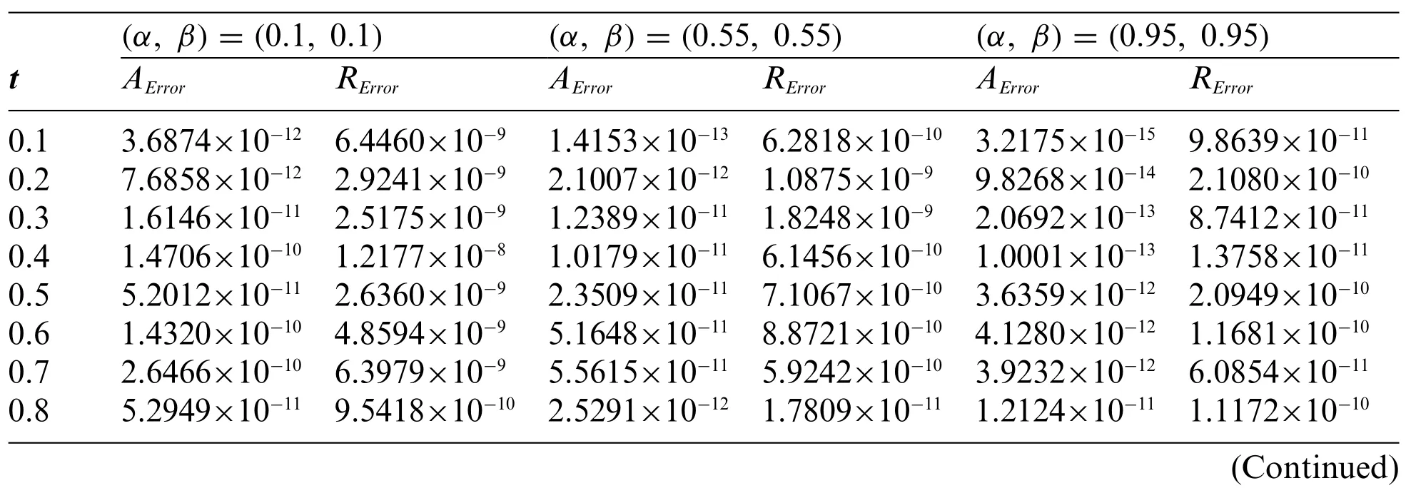
Table 1:The absolute and relative errors obtained for problem 1 using the Euler’s method for various values of α, β with ME =32

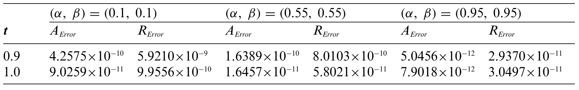
Table 1 (continued)

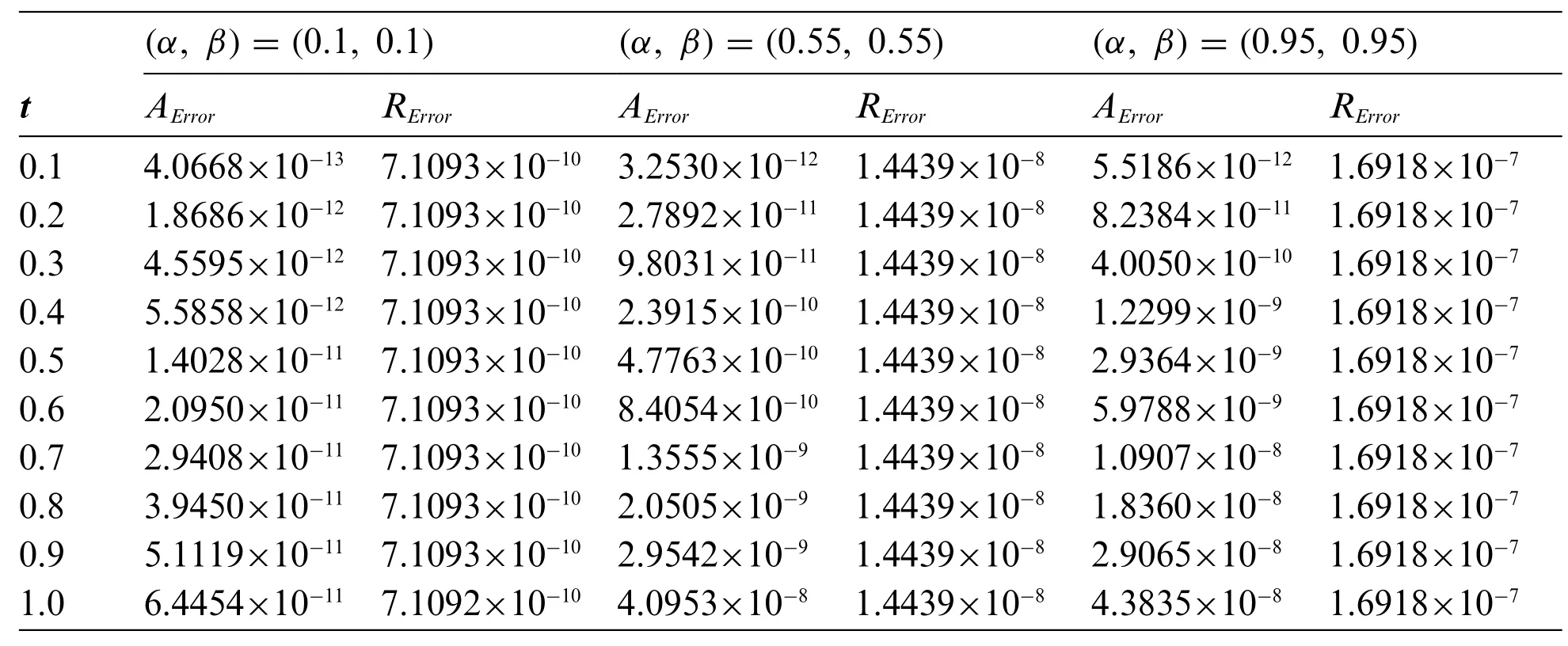
Table 2:The absolute and relative errors obtained for problem 1 using the Talbot’s method for various values of α, β with MT =26

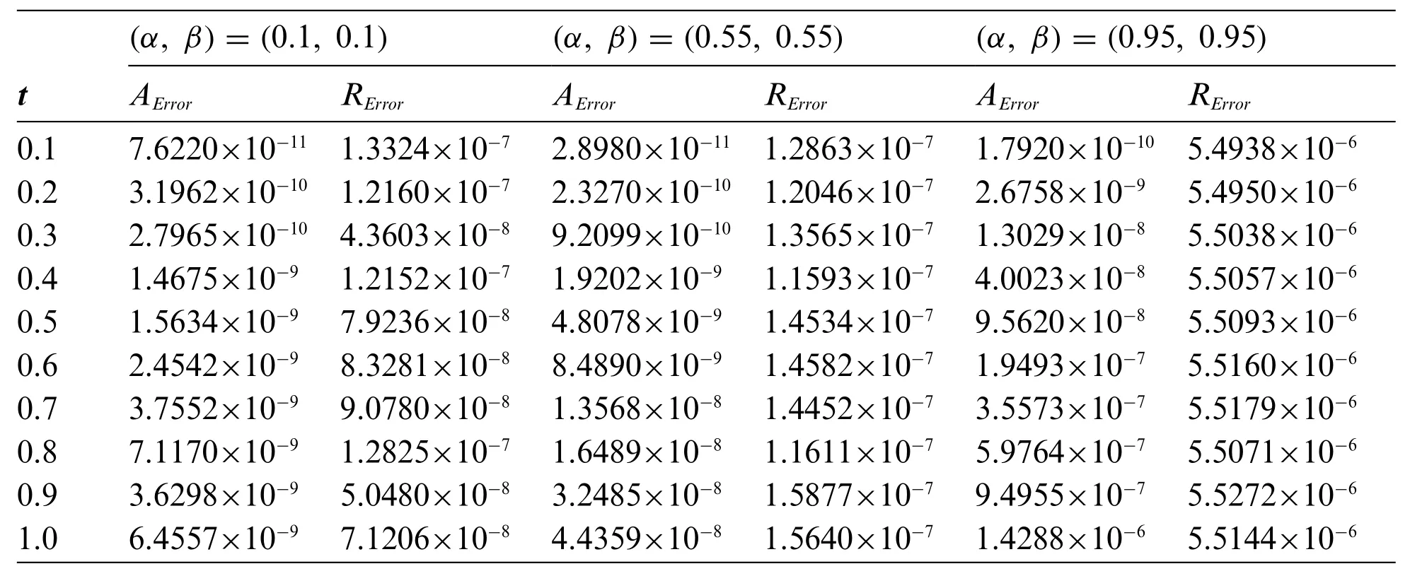
Table 3:The absolute and relative errors obtained for problem 1 using the Stehfest’s method for various values of α, β with MS =18

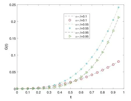
Figure 2:The plot shows the numerical(markers)and exact(dashed lines)solutions for various values of α, β using Talbot’s method with MT = 24.We can see that the numerical solutions have good approximations to the exact solutions

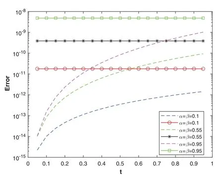
Figure 3: The plot shows the convergence rate of the relative errors (markers) and absolute errors(dashed lines)vs.time for various values of α, β using Talbot’s method with MT =26

Problem 2.

We consider a linear fractal fractional differential equation of the form

With exact solution

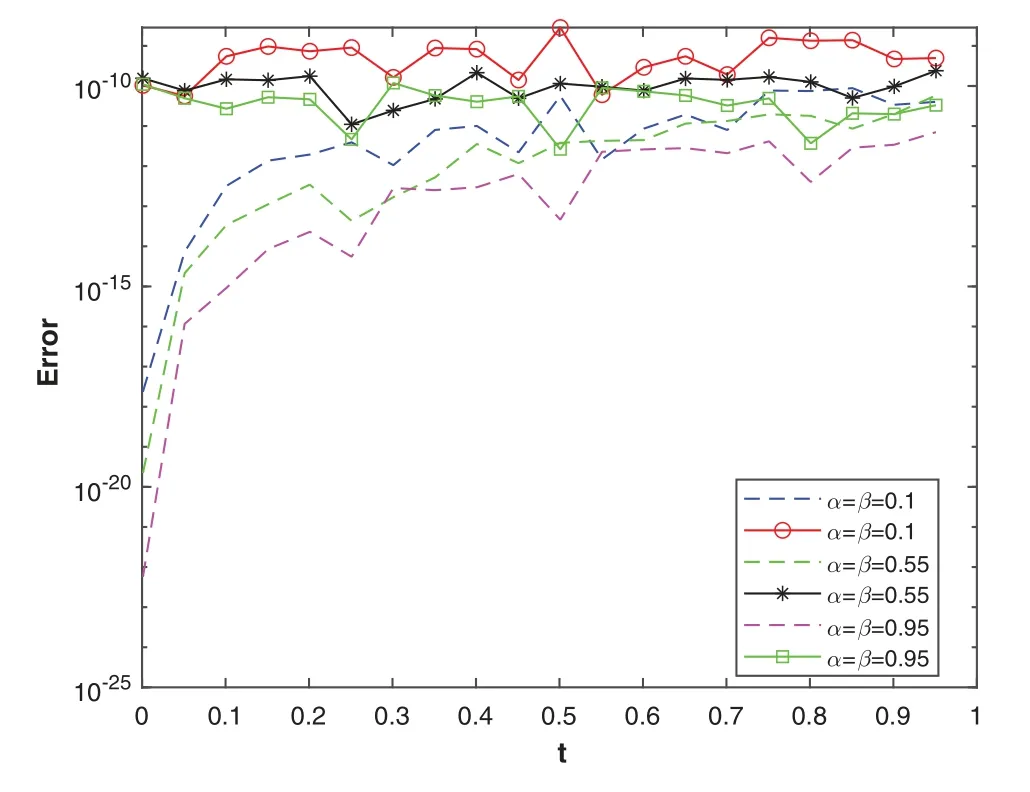
Figure 4: The plot shows the convergence rate of the relative errors (markers) and absolute errors(dashed lines)vs.time for various values of α, β using Euler’s method with ME =32

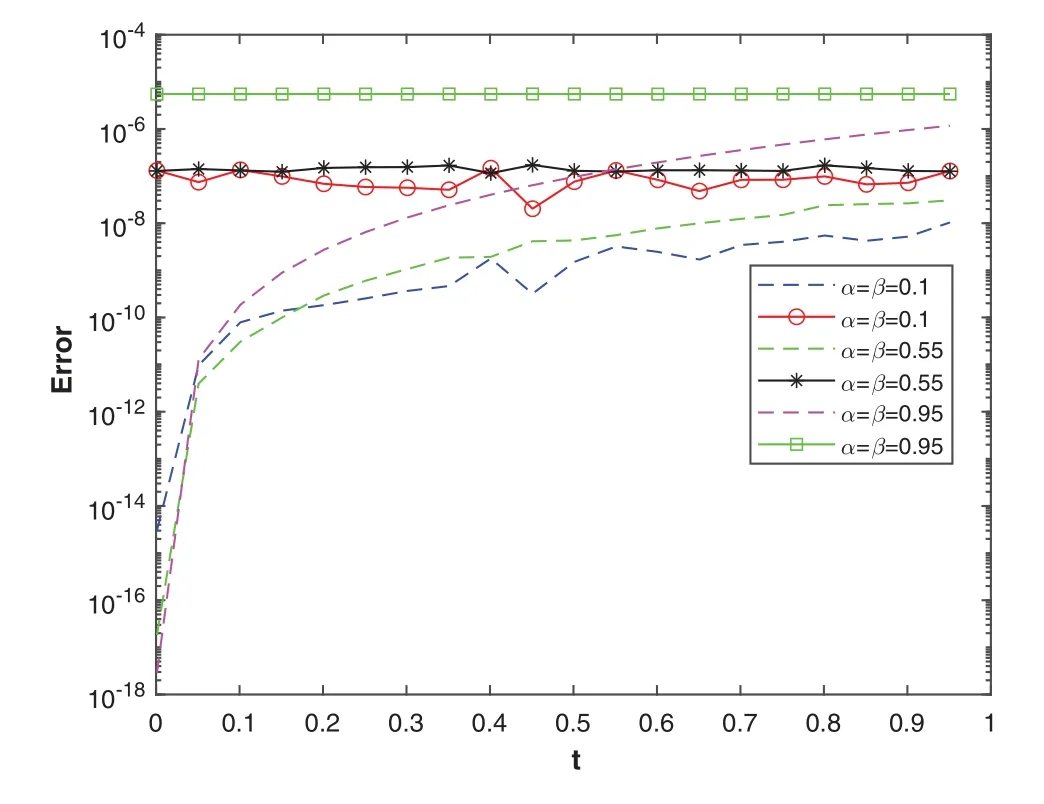
Figure 5: The plot shows the convergence rate of the relative errors (markers) and absolute errors(dashed lines)vs.time for various values of α, β using Stehfest’s method with MS =18

The problem is solved using three NILT schemes.In Table 4, the absolute and relative errors of the problem using the Euler’s method are displayed.Tables 5 and 6 show the results obtained using the Talbot’s and Stehfest’s methods for various values ofαandβ.Fig.7 shows the plots of numerical and analytic solutions for various values ofαandβusing the Talbot’s method.The plot of absolute and relative errors for different values ofαandβusing Euler’s method is shown in Fig.8.Fig.9 shows the plot of absolute and relative errors of the problem using Talbot’s method.In Fig.10,the absolute and relative errors for various values ofαandβusing Stehfest’s method are shown.Similarly in Fig.11,a comparison between the absolute errors using the three schemes is presented.It is clear from the figure that the Euler’s and Talbot’s methods performed better than the Stehfest’s method.

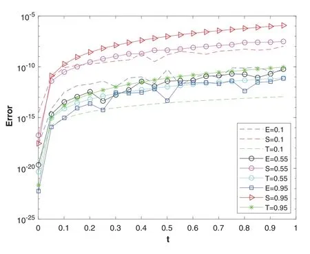
Figure 6: The plot shows the comparison of the convergence rate of the absolute errors of the three methods,Euler’s method with ME = 32,Stehfest’s method with MS = 18,and Talbot’s method with MT =28.E =0.1,S =0.1,T =0.1 refers to absolute error of Euler’s,Stehfest’s and Talbot’s method with α =β =0.1 respectively and similarly for others

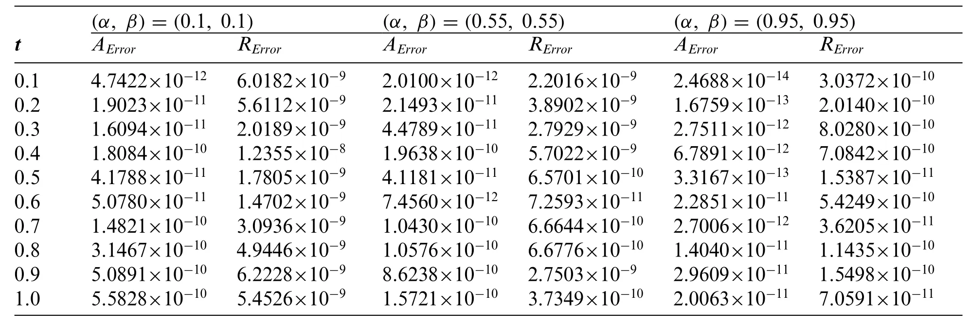
Table 4:The absolute and relative errors obtained for problem 2 using the Euler’s method for various values of α, β with ME =32

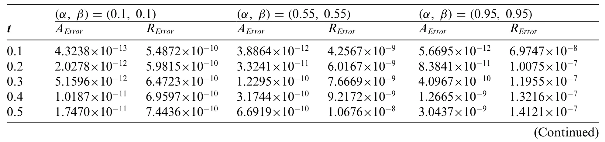
Table 5:The absolute and relative errors obtained for problem 2 using the Talbot’s method for various values of α, β with MT =24

Table 5 (continued)

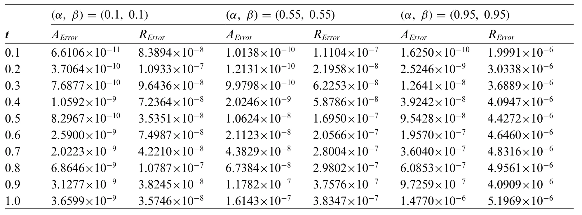
Table 6:The absolute and relative errors obtained for problem 2 using the Stehfest’s method for various values of α, β with MS =18

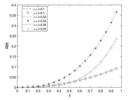
Figure 7: The plot shows the numerical solutions (markers) and exact solutions (dashed lines) for various values of α, β using Euler’s method with ME = 34.We can see that the numerical solutions have good approximations to the exact solutions

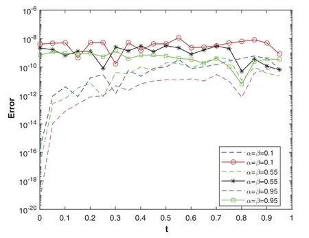
Figure 8: The plot shows the convergence rate of the relative errors (markers) and absolute errors(dashed lines)vs.time for various values of α, β using Euler’s method with ME =34

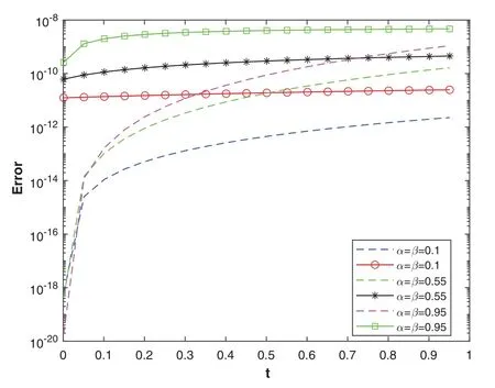
Figure 9: The plot shows the convergence rate of the relative errors (markers) and absolute errors(dashed lines)vs.time for various values of α, β using Talbot’s method with MT =26

Problem 3.

We consider a linear fractal fractional differential equation of the form

with exact solution

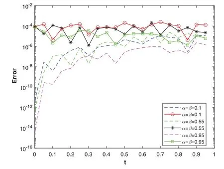
Figure 10: The plot shows the convergence rate of the relative errors (markers) and absolute errors(dashed lines)vs.time for various values of α, β using Stehfest’s method with MS =24

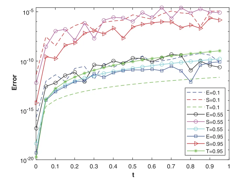
Figure 11:The plot shows the comparison of the convergence rate of the absolute errors of the three methods Euler method with ME = 34, Stehfest’s method with MS = 24, and Talbot’s method with MT =26.E =0.1,S =0.1,T =0.1 refers to absolute error of Euler’s,Stehfest’s and Talbot’s method with α =β =0.1 and similarly for others

The problem is solved using three NILT schemes.In Table 7, the absolute and relative errors of the problem using the Euler’s method are displayed.Tables 8 and 9 show the results obtained using the Talbot’s and Stehfest’s methods for various values ofαandβ.Fig.12 shows the plots of numerical and analytic solutions for various values ofαandβusing the Talbot’s method.The plots of absolute and relative errors for various values ofαandβusing Euler’s method are shown in Fig.13.Fig.14 shows the plots of absolute and relative errors of the problem using Talbot’s method.In Fig.15,the absolute and relative errors for various values ofαandβusing Stehfest’s method are shown.Similarly in Fig.16 a comparison between the absolute errors using the three schemes is presented.It is clear from the figure that the Euler’s and Talbot’s methods performed better than the Stehfest’s method.

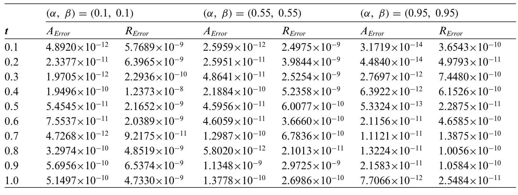
Table 7:The absolute and relative errors obtained for problem 3 using the Euler’s method for various values of α, β with ME =32

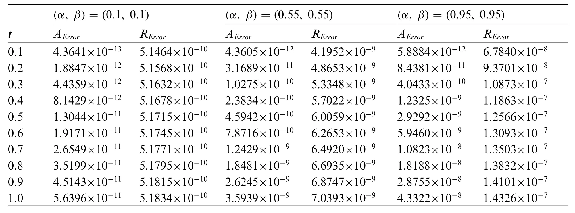
Table 8:The absolute and relative errors obtained for problem 3 using the Talbot’s method for various values of α, β with MT =24

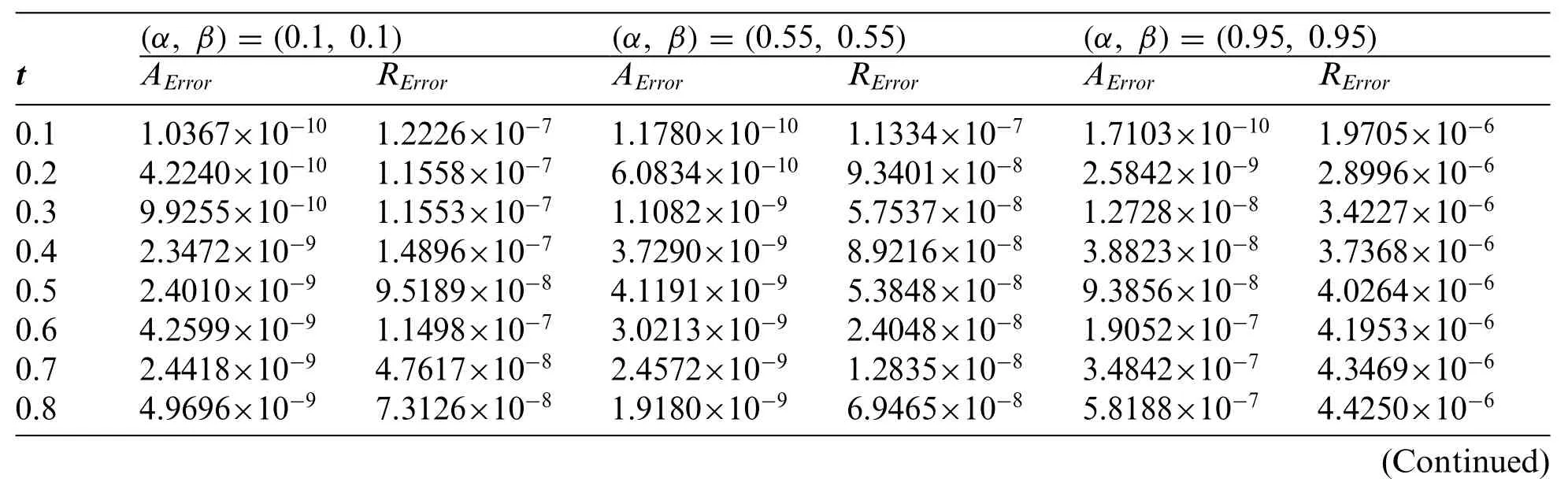
Table 9:The absolute and relative errors obtained for problem 3 using the Stehfest’s method for various values of α, β with MS =18

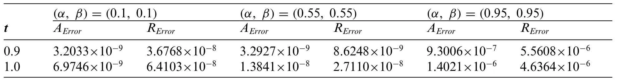
Table 9 (continued)

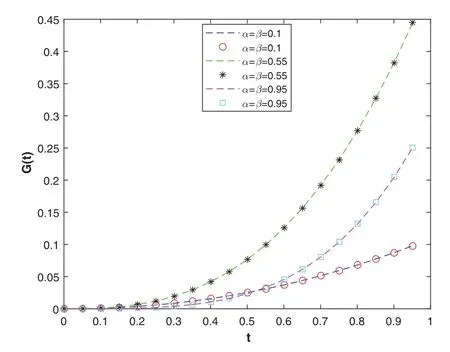
Figure 12: The plot shows the numerical solutions (markers) and exact solutions (dashed lines) for different values of α, β using Stehfest’s method with ME =26.We can see that the numerical solutions have good approximations to the exact solutions

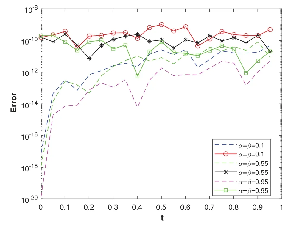
Figure 13: The plot shows the convergence rate of the relative errors (markers) and absolute errors(dashed lines)vs.time for various values of α, β using Euler’s method with ME =30

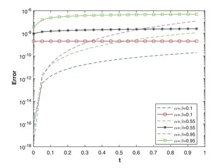
Figure 14: The plot shows the convergence rate of the relative errors (markers) and absolute errors(dashed lines)vs.time for various values of α, β using Talbot’s method with MT =22

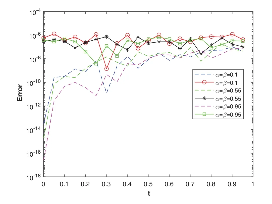
Figure 15: The plot shows the convergence rate of the relative errors (markers) and absolute errors(dashed lines)vs.time for various values of α, β using Stehfest’s method with MS =20

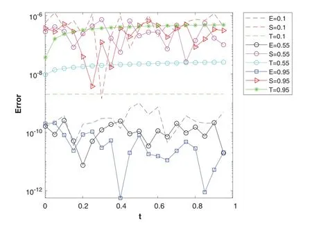
Figure 16:The plot shows the comparison of the convergence rate of the absolute errors of the three methods Euler method with ME = 30, Stehfest’s method with MS = 20, and Talbot method with MT = 22. E = 0.1,S = 0.1,T = 0.1 refers to absolute error of Euler’s, Stehfest’s and Talbot’s methods with α =β =0.1 and similarly for others

4 Conclusions

New concepts of differentiation and integration have been introduced recently.The new differentiation is a combination of fractal and fractional differentiation.In this paper,we have developed a Laplace transformed method for numerical modeling of fractal-fractional differential equations.In contrast to the standard finite difference method,the proposed method has used the Laplace transform and numerical Laplace inversion to handle the time fractal-fractional derivative.Solving differential equations of fractal-fractional order using time stepping technique may face the problem of timeinstability.However,this method avoids the time stepping method and hence the time-instability.We have utilized three Laplace transform inversion methods to evaluate the time domain solution for three fractal-fractional differential equations.In all cases,the inversion results have been proven excellent.All three inversion methods have produced accurate results.From the obtained results, it has been observed that Euler’s and Talbot’s methods are more accurate than Stehfest’s method.Furthermore,it has also observed that using Stehfest’s method,optimal accuracy can be achieved for values ofMSaround 20 or 22.Hence,the obtained results led us to the conclusion that these methods are excellent alternatives for approximating the solutions of such types of differential equations.It was also found that these inversion methods are applicable to such types of fractal-fractional differential equations.The proposed methods are easy to implement and highly accurate.

Acknowledgement:The authors K.Shah,T.Abdeljawad and B.Abdalla would like to thank Prince Sultan University for the support through the TAS Research Lab.

Funding Statement:The APC of this article is supported by Prince Sultan University.

Conflicts of Interest:The authors declare that they have no conflicts of interest to report regarding the present study.