
Application of Smoothed Particle Hydrodynamics(SPH)for the Simulation of Flow-Like Landslides on 3D Terrains
2023-03-12 09:00BinghuiCuiandLiaojunZhang
Binghui Cuiand Liaojun Zhang
1College of Civil and Transportation Engineering,Hohai University,Nanjing,210000,China
2College of Water Conservancy and Hydropower Engineering,Hohai University,Nanjing,210000,China
ABSTRACT Flow-type landslide is one type of landslide that generally exhibits characteristics of high flow velocities,long jump distances,and poor predictability.Simulation of its propagation process can provide solutions for risk assessment and mitigation design.The smoothed particle hydrodynamics(SPH)method has been successfully applied to the simulation of two-dimensional(2D)and three-dimensional(3D)flow-like landslides.However,the influence of boundary resistance on the whole process of landslide failure is rarely discussed.In this study,a boundary condition considering friction is proposed and integrated into the SPH method,and its accuracy is verified.Moreover,the Navier-Stokes equation combined with the non-Newtonian fluid rheology model was utilized to solve the dynamic behavior of the flow-like landslide.To verify its performance,the Shuicheng landslide event, which occurred in Guizhou, China, was taken as a case study.In the 2D simulation, a sensitivity analysis was conducted, and the results showed that the shearing strength parameters have more influence on the computation accuracy than the coefficient of viscosity.Afterwards,the dynamic characteristics of the landslide,such as the velocity and the impact area,were analyzed in the 3D simulation.The simulation results are in good agreement with the field investigations.The simulation results demonstrate that the SPH method performs well in reproducing the landslide process,and facilitates the analysis of landslide characteristics as well as the affected areas,which provides a scientific basis for conducting the risk assessment and disaster mitigation design.
KEYWORDS Flow-like landslides;smoothed particle hydrodynamics;non-Newtonian fluid;boundary treatment
1 Introduction
The occurrence of landslides is usually introduced by earthquakes or heavy rainfall,and is always accompanied by a large number of casualties and extensive damage[1].According to the classification of landslides,there is a term“flow-like landslides”,which has the characteristics of fast flow velocity and long run-out distance,that causes severe damage[2–4].Therefore,great attention should be paid to these flow-like landslides to study the flow mechanism and the sliding characteristics.Due to the vast scale,unpredictability,short duration,and destructive character of landslide disasters,it is quite difficult and dangerous to record the process in real-time.Numerical methods can simulate the flow behavior of such landslides,and can also be applied to the investigation and evaluation of landslides.Most numerical studies on landslides are based on solid mechanics analysis methods,such as the limit equilibrium,finite element method(FEM)[5]and the fracture mechanics method[6].These methods focus on slope stability analysis,which analyzes the mechanism of landslide damage from the stressstrain perspective.However,these methods are not able to simulate the large deformation state of the landslide,and thus cannot reproduce the whole landslide process.
For physical experiments, it is a very effective and straightforward way of observing landslide characteristics.However, large-scale landslide or debris flow experiments are very expensive and time-consuming.Recently, numerical simulations based on various numerical methods have been widely employed in the simulation of landslides[7].The discrete element method(DEM)is a feasible method for simulating landslides[8–10].DEM treats this geotechnical material as a collection of rigid particles governed by Newton’s laws of motion.The interactions between particles are represented through appropriate force-displacement relationships that relate to the overlap and contact forces that can occur between particles.However,sufficiently small-time steps are needed to avoid numerical instability,leading to high costs when simulating problems containing a large number of elements.To reduce the computational effort,the grain size in a typical DEM simulation is typically significantly larger than that in a real problem.Another viable approach is discontinuous deformation analysis(DDA)[11,12].Since DDA was proposed,it has undergone extensive modifications and enhancements to make it more suitable for a wide range of real engineering challenges [13–15].However, the characterization of fluid flow still needs further improvement[16].
Among the recent advanced numerical methods, SPH is a mesh-free method, a completely Lagrangian method in which the particles carry field variables,(such as mass,pressure,energy,etc.)and move with material velocity[17].Since it was first introduced in 1977 to solve astrophysical problems in three-dimensional open space[18,19],it has been widely used in different fields due to its meshless and Lagrangian nature.This method provides better robustness and reliability in solving large deformation simulations,owing to the absence of computational grids or meshes[20,21].Therefore,SPH is more suitable for the simulation of flow-like landslides [22].The SPH still has some inherent flaws, such as tensile instability,absence of consistency or completeness of interpolation,zero-energy mode,and treatment of boundary conditions, etc.[23].With the continuous improvement of the SPH method,the method has been successfully applied to geological hazards[2,4,24,25].Lots of literature[26–28]reported the successful simulation of flow-type landslides as non-Newtonian fluids using the SPH method in combination with the Bingham constitutive model.Most of the existing SPH simulations are based on two-dimensional analysis,which cannot reflect the diffusion and lateral shrinkage,which are different from practical applications.Moreover,the SPH method has recently become more popular,due to the remarkable progress in accuracy,such as the incompressible SPH[29],corrective smoothed particle method(CSPM),and Delta-SPH[30].
Boundary treatment has been the main focus and difficulty of the SPH method, which affects the accuracy and precision of the calculation.Many different approaches have been proposed in the literature to enforce the solid boundary conditions to prevent particle penetration [31–33].The proposal of a generalized wall boundary condition is an alternative to the dynamic boundary conditions, which can be applied in complex geometries [34,35].However, the current simulation of non-Newtonian fluids lacks the treatment of fluid-solid boundaries[36].The literature suggested that the application of free-slip boundary conditions to treat the fluid-solid boundary will make the non-Newtonian fluid unable to obtain resistance from the solid wall boundary in the simulation, thus making the simulation and experiment inconsistent[37].
In this study, a boundary treatment method is proposed that considers friction based on the SPH method.The boundary particle viscous force term is obtained by interpolating the values of the fluid particles near the boundary.In addition, the boundary treatment is verified by comparing the simulation results to the experimental data.The Cross model was employed in the SPH method to simulate the landslides.The rheological parameters were derived from the Bingham model and the Mohr-Coulomb criterion.As a case study,the effectiveness and stability of the application were verified by reproducing the Shuicheng flow-like landslide event in both 2D and 3D that occurred on 23 July 2019,in Guizhou Province,China.The simulation results were compared to the field survey data, showing that the SPH model can provide an accurate analysis of the kinetic characteristics of flow-like landslides,including the flow path,movement velocity,run-out distance and deposition.
2 SPH Method
2.1 Concepts of SPH
For the SPH method,the entire domain is represented as a set of randomly distributed particles with no connection between them.Two main steps are required to obtain the fluid governing equations in SPH form,namely,the kernel approximation and the particle approximation.Firstly,approximation of the field function and its derivative are derived from an integral representation method by using a smoothing kernel function.Secondly,these approximations are replaced by the sum of all neighboring particles in the support domain.It is the kernel approximation and particle discretization that make the SPH method work well for free surface flows and large deformations[17,38].
The integral representation of a functionf (x)may be given as the following kernel approximation using the smoothing technique:

wheref (x)is a field function of the three-dimensional position vectorx, andW(x-x′,h)is the smooth function.The smoothing length h that determines support domain Ω.The discrete form of a function at particleican eventually be described as:

wheremjandρjare the mass and density of particlej,respectively,andWij=indicates the smoothing function.In the same manner,the particle approximate form for the spatial derivative of the function can be formulated as:

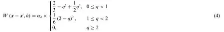
There are several kernel functions that are widely utilized.Typically,higher-order kernel functions often enhance the computing accuracy,and substantial time is required.The cubic spline kernel,which belongs to the B-spline family,is one of the kernels that is commonly employed in SPH method[17]and is given by:
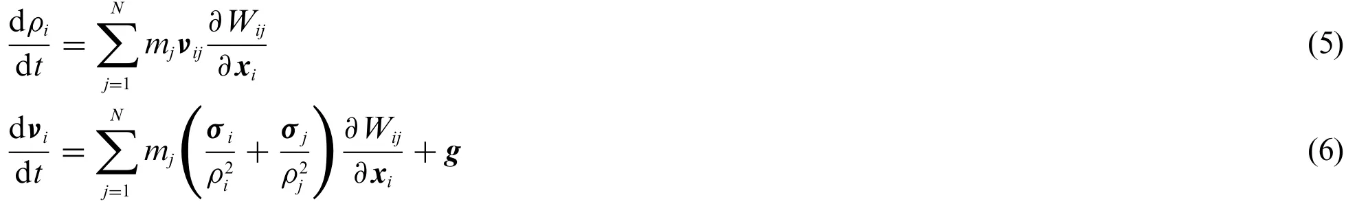
νij=indicates the velocity difference between particleiand particlej;σrepresents the total stress tensor andgis the gravity acceleration,respectively.
Due to the density approximation,the pressure field in the SPH formulation for weakly compressible fluids generally exhibits instability and numerical noise.Particularly,in the present case,the noise of the pressure field may be critical.In this study,the delta-SPH method[30]was adopted,which was implemented by adding a diffusive term in the continuity Eq.(5)and it can be written as:

whereξis the diffusive coefficient,which is usually adopted as 0.1;c0is the speed of sound at reference density;andψijis written as:

whereεhis a small constant and is usually adopted as 0.01.
Regarding the momentum Eq.(6), the total stress tensorσcan be written as the summation of an isotropic component pressure p and a viscous shear stress componentτ.To remove the numerical oscillations,the Monaghan type artificial viscosity Πijwas adopted in this study,which is most widely used in the current SPH simulation.After considering the artificial viscosity,the momentum equation can be written as:
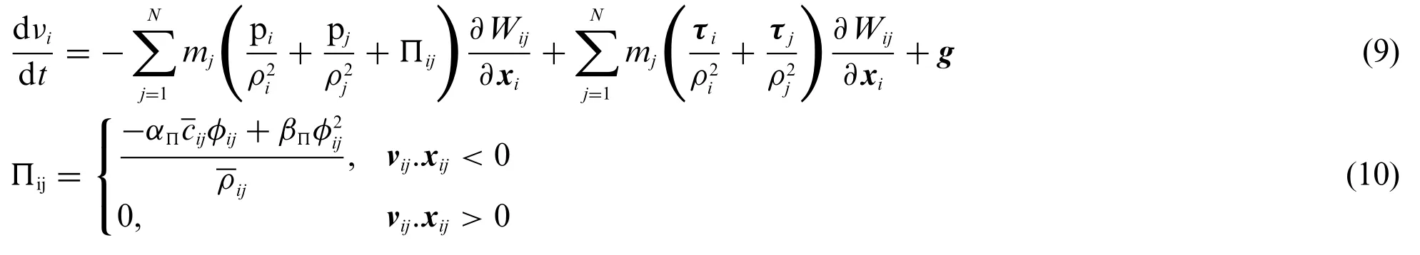
whereαΠandβΠare two constants and are commonly set as 0.1 and 0.01, respectively; Detailed parameter definitions can be found in reference[39].
In this work, the temperature of landslides is considered as a constant.Therefore, the energy equation is not considered.In the typical SPH method for resolving the compressible flows,the particle motion is governed by the pressure gradient, whereas the particle pressure is determined using an appropriate Equation of State(EoS).

whereγis commonly set to be 7.0;c0is the speed of sound and is commonly set at least 10 times the maximum fluid velocity for the sake of keeping the density fluctuation within 1% which can be calculated byβ(ghmax)1/2.βis a constant and is set as 10 in this study.
2.2 Rheological Model
PySPH is an open-source framework for the simulation of the SPH method [40].The original PySPH code(version 1.0b1)is able to handle with the free-surface flows,but it is incapable of dealing with non-Newtonian flows.A relevant constitutive model should be developed in the original code to allow for the landslide simulation.In Newtonian fluid dynamics,the shear stress of the fluid can be expressed by the following equation:


whereμeffis the effective viscosity that is changed over time.The effective viscosity of the Bingham model can be formulated as:

whereμBis the Bingham viscosity andτyis the yield stress,respectively.
Assuming that under the condition of shear rate, ˙γ→0,μeffin Bingham model approaches an infinite value,therefore,the direct application is not available.To solve this problem,existing studies employed a variety of strategies to avoid numerical divergence,i.e.,the simple regularization[42]and the threshold regularization[43].In this study,the general Cross model[44]was chosen to characterize the non-Newtonian behavior of flow-type landslides.

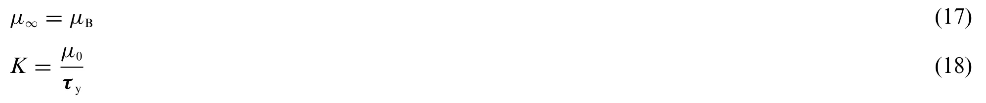
whereμ0andμ∞represent the fluid’s viscosity at extremely low and high shear rates,respectively;K and m are the constant parameters of the Cross model.For the sake of simplicity,the methodology in which these values are derived by incorporating the more commonly utilized Bingham fluid parameters was adopted [29].Assumingm= 1 in Eq.(15), the effective viscosity in the Cross model can be formulated as:

Typically,K˙γ >>1,by Eq.(14)with Eq.(16),the remaining two parameters in the Cross model can be given as follows:
The Mohr-Coulomb yield criterion with the cohesioncand frictional angleφ,which is adopted to describe the soil yielding process,is introduced into Eq.(12)[3],which can be written as:

whereσis the pressure in this status.Related literature[45]pointed out that the numerical solution’s accuracy is satisfactory as the viscosity at a low shear rate is 1000 times greater than that at a high shear rate.

Notice that the advantage of the Cross model over the Bingham model is that the effective viscosity is a continuous variable,and the numerical instability is avoided,as shown in Fig.1.
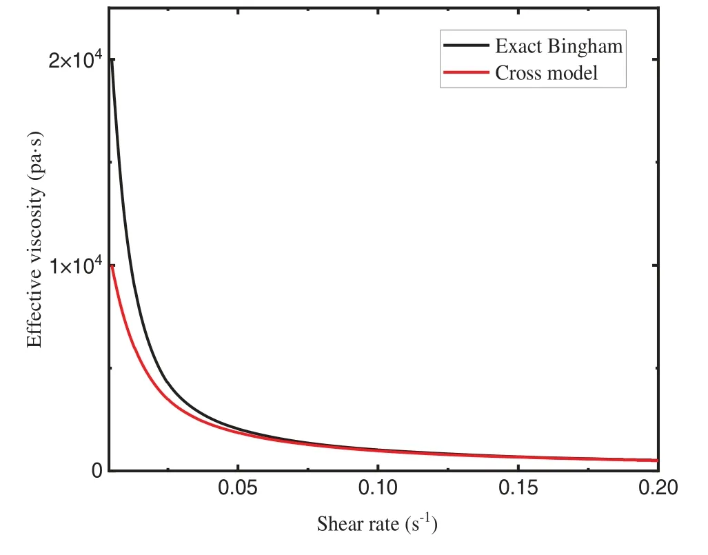
Figure 1: Effective viscosity against shear rate of different rheological model for parameters (μB =20 Pa·s,τ0 =100 Pa·s)
2.3 Boundary Condition
The boundary treatment has been a main challenge in SPH simulation and affects the calculation accuracy as well as the efficiency.It is vital to select an adequate boundary condition that represents the effect of solid boundary in order to closely describe the dynamic mechanism of landslides,as shown in Fig.2.
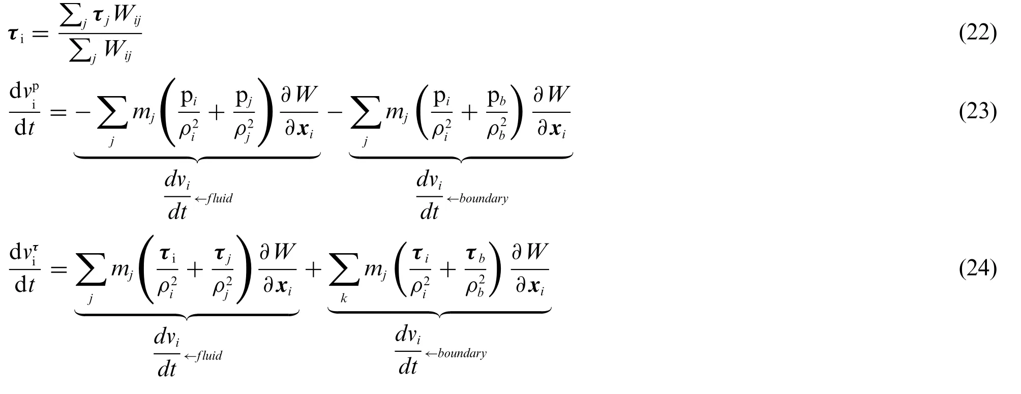
A simple and convenient boundary condition was proposed that can consider the boundary friction.In this work, two types of boundary conditions need to be set.Firstly, when a particle approaches to a solid boundary, the kernel function will be truncated, and an error in the solution result will occur.To address this issue,a generalized wall boundary condition by Adami et al.[46](see Eq.(23)),was introduced.By extrapolating from the neighboring fluid particles,the pressure on the solid boundary is obtained as:

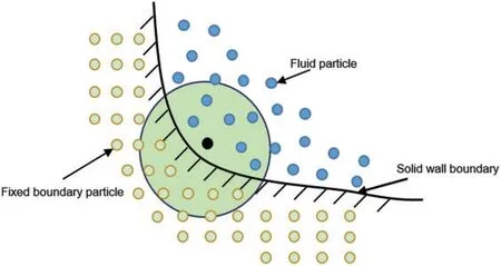
Figure 2:Illustration of the boundary condition
Secondly, the discrete particles of landslides may slip at the boundary and thus suffer from the slippage resistance (see Eq.(24)).Referring to the concept of pressure interpolation on the solid boundary,the value of the viscosity force on the solid boundary was given by:
Through the above two steps, the no-slip boundary conditions considering friction on the solid boundary was successfully set.When calculating the viscous forces on the boundary,both the dynamic viscosity coefficient can be obtained by interpolation from the fluid,or a fixed viscosity coefficient can be set.
2.4 Time Integration Schemes
Prediction-correction algorithm was adopted to execute the time integration.For continuity equations and momentum equations of the form,all the values of time-variant quantities are predicted at the time stepn+1,based on the time stepn+1/2,as follows:

Afterwards,these values are updated at another half time step:

At the end of the time step,the values are calculated as follows:

The selection of the magnitude of time stepΔtis limited due to the stability reasons based on several criteria: the Courant Friedrichs Lewy (CFL) condition, the force terms, and the viscous diffusion terms,as follows:

The flow chart of the SPH with proposed boundary condition is shown in Fig.3.
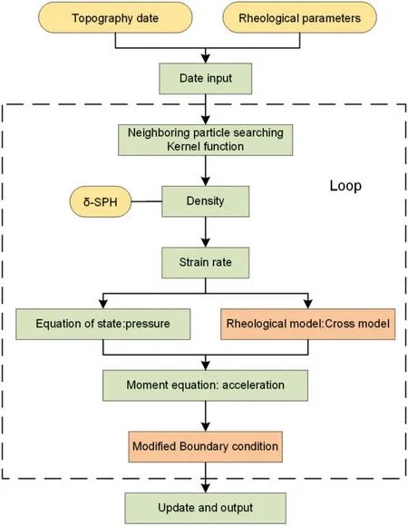
Figure 3:The flow chart of the SPH with proposed boundary condition
3 Verification of the SPH Model
In this section,the proposed boundary condition coupled SPH model is utilized to simulate the granular flow model test conducted by Moriguchi et al.[47] to verify its numerical accuracy.Fig.4 shows the configuration of the granular flow model.The test was conducted in a tank with the dimensions 300 cm×50 cm×50 cm for length,height and depth,and an instrument with 3 cm height was fixed in the bottom of the tank for measuring the impact force.The bottom surface of the tank is coated with the same sand to provide surface friction,but the side surfaces of the walls were considered smooth.One of the side walls of the tank was made of acrylic sheets to allow detailed observation of the flow behavior of the dry sand with a video camera.After the sliding door was opened,the flowing distances of the mortar sample were recorded with a video camera at a certain time interval.
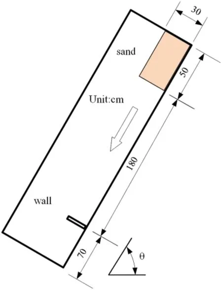
Figure 4:Schematic of the sand flow model test
Two different flume inclinations were chosen for the two-dimensional simulation, and the parameters are given in Table 1.Each flume inclination is divided into two cases.One case is that the proposed boundary condition is applied to the bottom of the slope.Another case is that the freeslip boundary is applied to all the walls.As the simulation proceeds,a large number of sand particles have a tendency to move from the right side to the left side due to the effect of gravity.Then,the sand particles start to accelerate and hit the measuring wall.
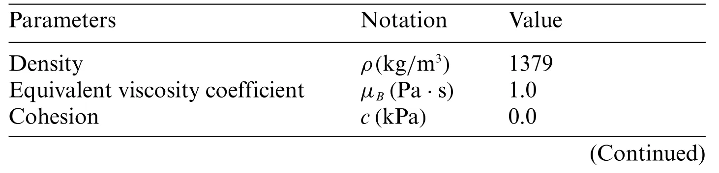
Table 1: The input parameters of numerical simulations
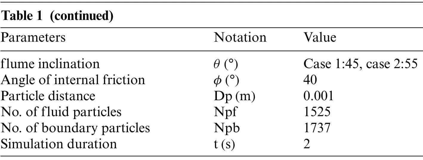
Table 1 (continued)Parameters Notation Value flume inclination θ(°) Case 1:45,case 2:55 Angle of internal friction φ(°) 40 Particle distance Dp(m) 0.001 No.of fluid particles Npf 1525 No.of boundary particles Npb 1737 Simulation duration t(s) 2
The simulation process with the flume inclination ofθ= 45° is presented in Fig.5.Simulation results show that the model can reasonably simulate the flow behavior of sand.Figures suggest that flume inclination ofθ=45°were small enough to allow the sand to overtop the wall.However,sand was easy to get over the wall with the free-slip case.On the other hand,flume inclination ofθ= 55°would be so high for the sand to over the wall,as the numerical solution simply predicted that a part of the sand of would come to rest in the back of the wall.
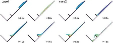
Figure 5:The simulation process of the sand flow model test(case 1:the proposed boundary condition,case 2:the free-slip boundary condition)
To quantitatively analyze the impact of the boundary,the impact force of the flowing sand was measured for different flume inclinations and different boundary conditions.The simulated time histories of the impact force of the flowing sand are presented in Fig.6.Comparing the results with the tested data,these two figures show that the peak impact force value of impact forces can be well captured by the SPH model.As excepted,comparing different boundary cases,the peak impact force generally agrees well with the tested data when the friction boundary is considered.
4 Case Study
4.1 Geological Setting and Flow-Like Landslides Features
The Shuicheng flow-like landslide event was triggered by intense rainfall in July 2019 (Fig.7a).A total of three heavy rainfall events occurred in the week before the occurrence of landslides, with a cumulative rainfall of 288.9 mm.Under the influence of continuous heavy rainfall, the landslide began to lose stability and rapidly slid along the slope at high speed.After roughly 700 m of landslide movement, two diversions were formed after hitting a small ridge and subsequently impacting and burying the residential buildings on the lower part of the slope.The mass flow of landslide spread along the slopes for about 1490 m and was deposited in the gully depressions.Due to the suddenness of the landslide and the lack of protective measures such as blocking,the disaster destroyed 21 houses and 43 people were killed.
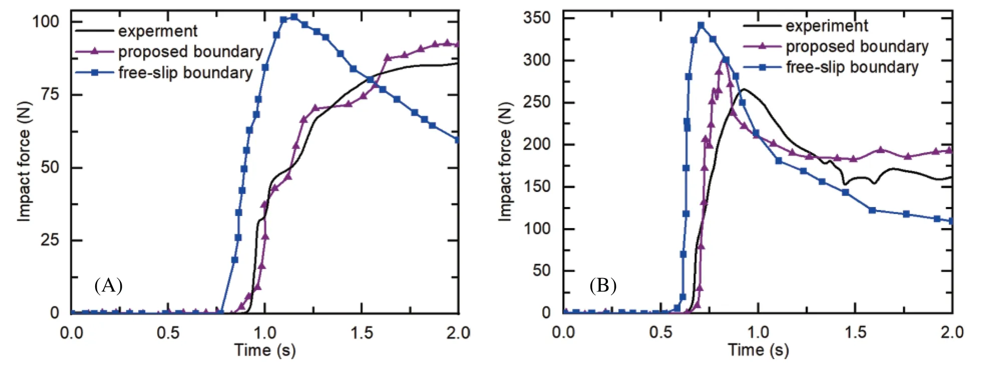
Figure 6:Simulated time histories of impact force for different flume inclinations(A:45°,B=55°)
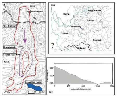
Figure 7:The 2019 Shuicheng flow-like landslide event(a)location of the Shuicheng(b)scope of the landslide(c)typical cross-section of the Shuicheng gully
The Guizhou Provincial Geological Disaster Emergency Technical Guidance Center immediately carried out the field investigations following the occurrence of landslide.The primary characteristics of the flow-like landslides are depicted in Fig.7b as well as a typical cross-section of the Shuicheng gully in Fig.5c.According to the field investigations, the entire landslide is approximately 1300 m long,with a large distance of around 460 m between the front and rear edges,and a volume of about 191.2×10⁴m3.According to Zhou et al.[48],the average density of the Shuicheng landslide mass was about 2000 kg/m3.Depending on the test results,the angle of internal friction and the cohesion of the flow-like landslide can be set approximately as 30°and 30 kPa,respectively.In the previous simulations,the Bingham model was widely applied to simulate the landslides or debris flows considering a range of dynamic viscosities from 20 to 500 Pa ·s [49].In this work, the empirical physical experimental equation is used to obtain the dynamic viscosities[50],which is given below:

whereCvis the volume concentration.According to the investigation report,the best-fittedCvis 44%,resulting in a dynamic viscosity of 255 Pa·s.
According to the simulation results, the whole process duration was about 90 s.Fig.8 presents the slope configurations at different time points,reflecting the movement of landslides.The particles slipped down from the top of the landslide and then moved along the steep slope by gravity.Finally,these particles reached an equilibrium state and were deposited in the lowlands.The overall performance of the sliding was accelerated motion in the period 0–30 s and decelerated motion after 30 s.
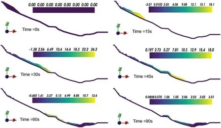
Figure 8:Two-dimensional simulated results for the motion process of Shuicheng landslide
Landslides usually have a long distance,and the measurement and selection of various parameters may vary greatly in different locations.Therefore, it is meaningful to conduct a sensitivity analysis to determine how various rheological parameters affect the simulation results.Table 2 lists the eight calculation cases with different rheological parameters.To explicitly quantify the differences of the sensitivity of different parametersεv,was evaluated using the following equation:

whereΔvjis the velocity difference between case j and case 1,and N=18 represents the number of velocity at an interval of 5 s.The results of all the eight cases are presented in Table 2 and Fig.9,which show that the internal friction angle has more influence on the computation accuracy in comparison with the cohesion of landslides.
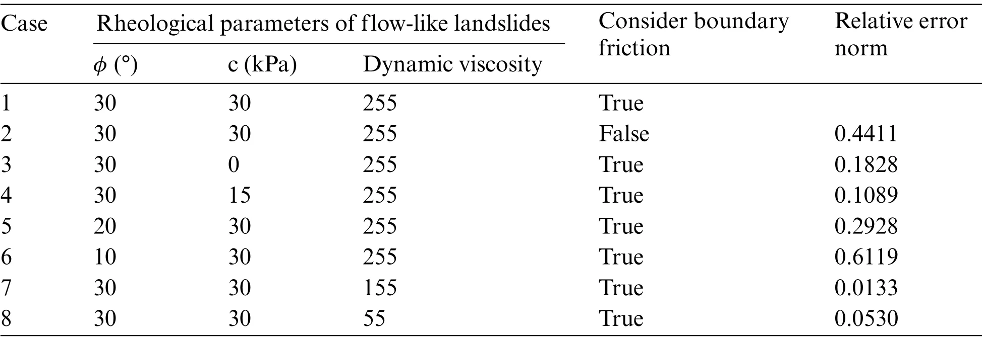
Table 2: Relative error norm in the velocity
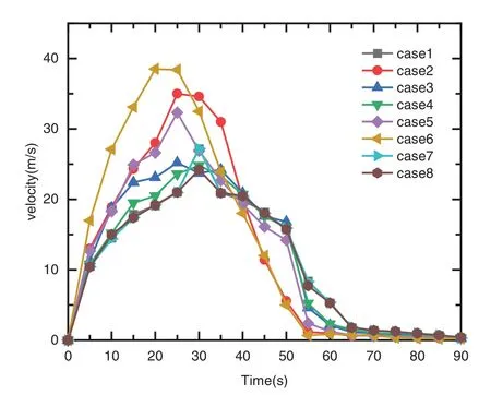
Figure 9:Velocity–time history curves of different cases
4.2 Three-Dimension Modeling
Since the 2D simulation cannot reflect the diffusion and lateral contraction, 3D simulation on the real complex terrain is necessary.In this section, the 3D terrain is generated from the original topographic map at a scale of 1/2000 and homogenizes the mesh.The previously created mesh is then transformed into a sequence of boundary particle particles.Similarly,the landslide is discretized into a succession of particles each with its own set of properties.In this simulation,the particle distance is set to 7.5 m,resulting in 12825 boundary particles and 7010 fluid particles.The strength parameters adopted in the 3D simulation are the same as in the 2D simulation (Table 3).Based on this model,Shuicheng landslide was numerically simulated in 3D terrain, and the results are shown in Fig.10.The color of the particles in the figures represents the sliding velocity at various instants.
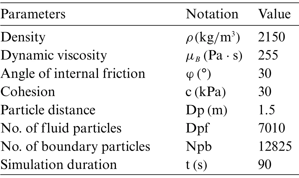
Table 3: Parameters run in the simulation of the Shuicheng landslide
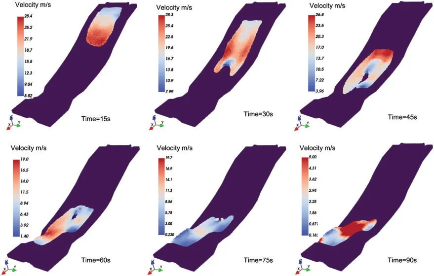
Figure 10:Snapshots of the Shuicheng landslide motion in different instants
The results suggest that the front flow takes about 28 s to travel nearly 520 m to reach the isolated island.The front flow velocity reaches a maximum with an average velocity of 29.8 m/s.Due to the good stability of the soil near the isolated island,it diverts the debris to the sides and forms a divergence.The diversion of the stable slope protects the lower residential houses and creates an“island of safety”.The existence of isolated islands has dramatically slowed down the landslides.Therefore,the front flow remains stable at about 90 s and is deposited in the lowlands.Eventually,the estimated total volume of deposition is 1.1×10⁶m3,which is less than the field investigation value 1.91×10⁶m3.The reason might be that the simulation process does not take into account the entrapment process.In addition,the simulated landslide paths and deposited areas matched well with the results of field investigations.The topographic data, in this case, were obtained from the 1/2000 scale topographic map, and it is considered that more accurate topographic data would help to obtain better simulation results.
The displacement and velocity time histories of the landslide front and rear were investigated to gain a better understanding of the landslide characteristics in the present simulation.Fig.11 depicts the velocity time series of the landslide’s front and rear.At around 20 s and around 45.5 s after failure,the flow-like landslide front and rear reach a maximum velocity of 29.2 and 26.5 m/s, respectively.Afterwards,an isolated island was encountered,the landslide diverged and the path was changed,and the speed gradually decreased.After moving for 70 s,the landslide came to a halt and was deposited in a lower area.It should be noted that the changes in velocity at various moments represent the complexity of the 3D terrain.Fig.12 shows the maximum displacements of the front and rear during the motion were 1099 and 859 m,respectively,at the time of 90 s after failure.Ma et al.[51]conducted extensive field investigations and calculated the maximum velocity of 25 m/s2,and a landslide duration of 60 s using the empirical equations.Both values turned out to be slightly smaller than the simulated results.Quantitative validation of the landslide simulation based on the field measured data and empirical equations were challenging.The error may be triggered by a combination of natural and artificial reasons, which makes the simulation more challenging.In addition, it can be seen that the flow’s pressure field is formed smoothly.Fig.13 depicts the evolution of the flow-like landslide pressure field over time.As previously stated,delta-SPH successfully corrects pressure field noise,particularly for the high viscosity fluids.
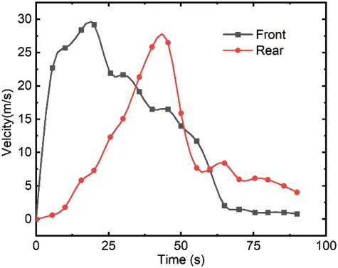
Figure 11:Velocity time history for front and rear of Shuicheng landslide
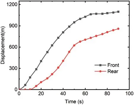
Figure 12:Displacement time history for front and rear of Shuicheng landslide
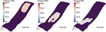
Figure 13:Pressure field of the Shuicheng landslide in different instants
The landslide material is discretized into a succession of SPH particles of almost the same diameters in this model.The greater the number of particles and the narrower the particle spacing,the greater the computing time required.It should be mentioned that, in the current code, the SPH module is accelerated based on Open Multi-Processing(OpenMP).In theory,the higher the number of particles in the SPH,the more accurate the simulation will be,but a balance needs to be reached with the needed calculation time.Fig.14 depicts the relationship between the program runtime and thread count.The results show that the computational efficiency of the proposed SPH model improves as the number of threads increases.Although the OpenMP code is more computationally efficient than the serial code on the CPU,the computation time consumption is large when more particles exist.
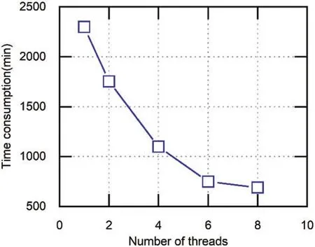
Figure 14:Relationship between computing time and number of threads in 3D SPH model
5 Conclusions
A rational simulation of flow-like landslide propagation process contributes to hazard analysis and disaster mitigation design.In this study, the Navier-Stokes equation combined with the non-Newtonian fluid rheology model was utilized to investigate the dynamic behavior of the flow-like landslide.
1.A simple and convenient boundary condition was proposed that can consider boundary friction.By using the proposed boundary condition, the simulation results are in good agreement with the experimental results.Moreover,since this operation is limited to boundary particles,it will not increase the computational overhead.
2.The Shuicheng flow-like landslide,which occurred in Guizhou in 2019,was studied as a case.The parameter sensitivity is analyzed under the 2D model,and the results show the shearing strength parameters have more influence on the computing accuracy than the coefficient of viscosity.
3.A 3D model of Shuicheng landslide was constructed and computed that corresponded to the site conditions.In terms of the solid volume and deposition area, the computed results are generally consistent with the field investigations.In addition, the characteristics of the front and the rear flow velocity and zone of influence of the flow-like landslide were analyzed,which will help the mitigation or countermeasure design work and offer evidence for the hazard assessment.
4.The approach provides an effective tool for studying the dynamic behaviors of landslides.However, the current study does not take into account the entrainment process of flow-like landslides.Large-scale practical problems usually require massive particles,and future research should be directed to GPU-accelerated modules.
Acknowledgement:The authors appreciate the valuable discussions with Zhang Weijie (College of Civil and Transportation Engineering, Hohai University, China) and Shi Wenbin (College of Civil Enginnering,Guizhou University,China)on topics of landslides.
Funding Statement:The authors received no specific funding for this study.after this line.
Conflicts of Interest:We declare that we do not have any commercial or associative interest that represents a conflict of interest in connection with the work submitted.
 Computer Modeling In Engineering&Sciences2023年4期
- Computer Modeling In Engineering&Sciences的其它文章
- A Study of BERT-Based Classification Performance of Text-Based Health Counseling Data
- Overview of Earth-Moon Transfer Trajectory Modeling and Design
- CEMA-LSTM:Enhancing Contextual Feature Correlation for Radar Extrapolation Using Fine-Grained Echo Datasets
- The Class of Atomic Exponential Basis Functions EFupn(x,ω)-Development and Application
- Corpus of Carbonate Platforms with Lexical Annotations for Named Entity Recognition
- Unique Solution of Integral Equations via Intuitionistic Extended Fuzzy b-Metric-Like Spaces