Seismic Liquefaction Resistance Based on Strain Energy Concept Considering Fine Content Value Effect and Performance Parametric Sensitivity Analysis

Nima Pirhadi,Xusheng Wan,Jianguo Lu,Jilei Hu,Mahmood Ahmad and Farzaneh Tahmoorian

1School of Civil Engineering and Geomatics,Southwest Petroleum University,Chengdu,610500,China

2Key Laboratory of Geological Hazards on Three Gorges Reservoir Area,Ministry of Education,China Three Gorges University,Yichang,443002,China

3College of Civil Engineering&Architecture,China Three Gorges University,Yichang,443002,China

4Department of Civil Engineering,Faculty of Engineering,International Islamic University Malaysia,Jalan Gombak,Selangor,50728,Malaysia

5Department of Civil Engineering,University of Engineering and Technology Peshawar(Bannu Campus),Bannu,28100,Pakistan

6Central Queensland University,Queensland,4740,Australia

ABSTRACT Liquefaction is one of the most destructive phenomena caused by earthquakes, which has been studied in the issues of potential,triggering and hazard analysis.The strain energy approach is a common method to investigate liquefaction potential.In this study,two Artificial Neural Network(ANN)models were developed to estimate the liquefaction resistance of sandy soil based on the capacity strain energy concept (W) by using laboratory test data.A large database was collected from the literature.One group of the dataset was utilized for validating the process in order to prevent overtraining the presented model.To investigate the complex influence of fine content(FC)on liquefaction resistance,according to previous studies,the second database was arranged by samples with FC of less than 28% and was used to train the second ANN model.Then, two presented ANN models in this study,in addition to four extra available models,were applied to an additional 20 new samples for comparing their results to show the capability and accuracy of the presented models herein.Furthermore,a parametric sensitivity analysis was performed through Monte Carlo Simulation (MCS) to evaluate the effects of parameters and their uncertainties on the liquefaction resistance of soils.According to the results,the developed models provide a higher accuracy prediction performance than the previously published models.The sensitivity analysis illustrated that the uncertainties of grading parameters significantly affect the liquefaction resistance of soils.

KEYWORDS Liquefaction resistance; capacity strain energy; artificial neural network; sensitivity analysis; Monte Carlo Simulation

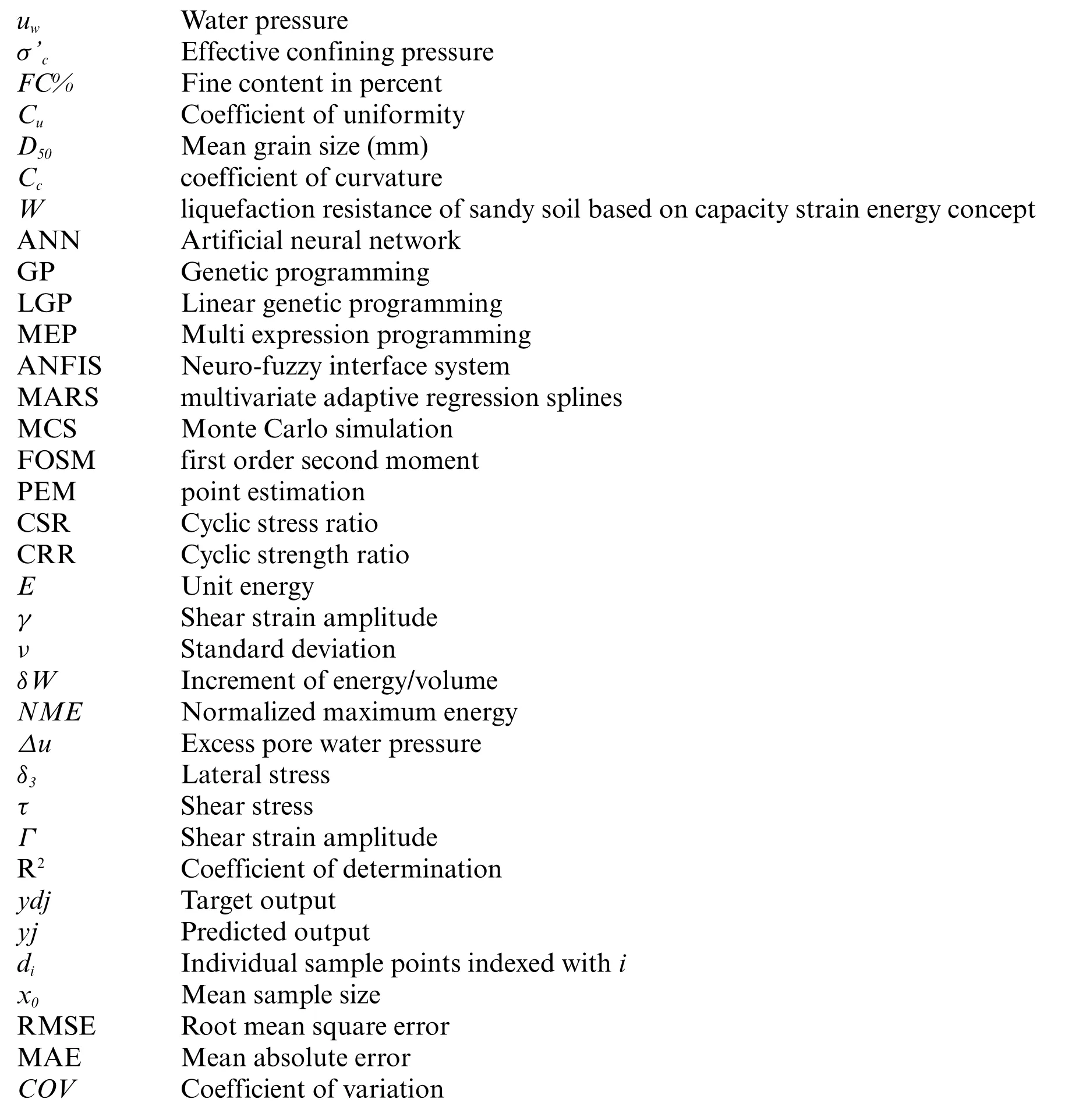
Nomenclature

1 Introduction

When saturated sand is subjected to an earthquake,because of the rapid vibrations,drainage is prevented and the tendency towards volume reduction,causes the transfer of the effective overburden stress to the pore water until excess pore water pressure becomes equal to the initial effective overburden stress;after which liquefaction happens.The most commonly reported liquefaction manifests in saturated loose or medium sandy soil have been observed during the most massive earthquakes worldwide.The 1964 magnitude 9.2 earthquake in Alaska and the magnitude 7.6 earthquake in Niigata of the same year, prompted extensive research on this phenomenon.Soil liquefaction has also been observed in recent earthquakes in China[1],Japan[2],Indonesia[3]and the USA[4,5].

Three main methods have been employed in relevant studies.The first one is the stress-based method,which was introduced by Seed et al.[6].And other researchers performed research to develop models using in-situ tests[7–9],laboratory tests[10,11]and numerical simulation[12–19].Additionally,the strain-based method was first introduced by Dobry et al.[12].They assumed under cyclic loading approximately 0.01% for threshold strain and initial water pressure (uw) increasing.After that, the shear strain was compared with 0.01 according to Serikawa et al.[2]or 0.02[3].Next,water pressure was estimated through experimental graphs.In the end,this water pressure was compared to confining stress to predict the triggering of liquefaction.In other words,depending on the following condition,liquefaction may or may not occur:

uw ＞σv0liquefaction occurs.

uw ＜σv0liquefaction does not occur.

whereσv0is initial vertical effective stress.

The coupled numerical models, since 1975, have been presented [13–17] based on Biot’s theory[18–20]which was the clarification of effective stress concept and coupled phases interaction between solid porous materials and fluid.Recently, some numerical simulation was also performed by researchers[21–28].The fourth method includes strain energy-based methods developed by applying seismic energy dissipated in the soil[21–30].This method has been applied in three main procedures by researchers which are using histories of site exploration liquefied[29–31],and laboratory test results[23,27,29–40] and Arias intensity-based models [32,41].To evaluate the potential of liquefaction in energy concept method,the capacity strain energy(W)value of the soil is required to be estimated to compare with the energy transferred to the soil by the earthquake loads.Since the energy dissipated by mechanisms(e.g.,cohesion and frictional mechanisms)cannot be easily discerned from laboratory and field data,the energy dissipated by frictional mechanisms is estimated by the total dissipated energy as the frictional mechanisms are expected to be dominant growing interest in earthquake engineering.In addition, the total amount of dissipated energy to the liquefaction point should be relatively independent of the sequence for increasing the load.On the contrary,the viscous mechanisms of energy dissipation can be considered for the low increase of strains where the rate of energy dissipated by this mechanism is directly related to the sequence used.In order to enhance the conventional load, the dissipated energy is expected to be greater than the liquefaction point,which is either independent or increases due to the load sequence used.

Based on laboratory test results six input parameters including effective confining pressure(σ’c)kPa, initial relative density (Dr)%,FC%,coefficient of uniformity (Cu), mean grain size (D50) (mm)and coefficient of curvature(Cc),have been identified and confirmed as the most influential factors in modeling liquefaction to estimate liquefaction resistance of sandy soil based on capacity strain energy concept[23,27,29–40].Clearly,permeability of the soil is considered implicitly in soil properties parameters ofDr,Cu,D50andCc.

These studies,except Cabalar et al.[37],extractedCcin their final correlation due to its limited range values in the datasets and hence,its limited effect.Furthermore,they included all ranges of the parameters in their models without special consideration to their value.

Further, Maurer et al.[42] analyzed 7,000 case histories from Canterbury Earthquakes in 2010–2011 and concluded when soils contain a high value ofFC, assessment of liquefaction is less reliable.Zhang et al.via laboratory tests showed that liquefaction potential is closely related toFC[38].Liu et al.[43] performed some experimental tests on marine sediments and proposed a critical value forFCto evaluate liquefaction resistance.Additionally,Tao[44]defined the limit value of 28%for estimating the liquefaction resistance, and through laboratory test results showed liquefaction resistance becomes more dependent onDrwhenFCis higher than 28%,rather thanFCvalue.While,in all presented models there has not been consideration to different effect ofFCin different range.

Regarding the evaluation of liquefaction strength by applying the strain energy approach,several models have been developed using artificial neural network(ANN)[35], genetic programming(GP)[45,46],multi expression programming(MEP)[46],neuro-fuzzy Interface system(ANFIS)[37],and multivariate adaptive regression splines(MARS)[38].Although the importance of the validating phase has been indicated by many researchers[47–49],in all studies,data division was performed randomly in two groups of testing and training phases,without considering the statistical characteristics of the data.Also,no validating phase has been performed in order to avoid overtraining of the models.

Due to the uncertainty of geotechnical problems, particularly, liquefaction phenomena, some studies,such as Bayesian methods,have been performed to develop probabilistic forms and reliability analysis to evaluate the potential of liquefaction[50–56].Furthermore,artificial intelligence [57–63]and Monte Carlo simulation(MCS)which is a classic approach to assess risk in quantitative analysis,has recently been used in engineering and sciences[64–71]and also in the evaluation of liquefaction potential[72–74].Jha et al.[73]presented the probability of liquefaction due to factor of safety using FOSM method,an advanced first-order second-moment(FOSM),Hasofer–Lind reliability method,a point estimation(PEM),and an MCS method.They presented a new combined method using both FOSM and PEM to find the cyclic stress ratio(CSR)and cyclic strength ratio(CRR)statistically.They showed that the factor of safety measured by the combined method is similar to the PEM and MCS methods.They also indicated FOSM,PEM,and MCS methods present nearly the same probabilities of liquefaction by considering input variability.Using the jointly distributed random variables method and using the data from triaxial test results, Johari et al.[74] presented a reliability assessment of liquefaction and compared the results with the Monte Carlo simulation.The results exhibited close probability density functions of the safety factor applying both methods.

In this study, to investigate the complex effect ofFCon liquefaction resistance of soil in terms of the unit energy, two datasets were arranged.The first dataset was collected from the literature as the largest and likely most complete dataset employed by researchers covering a large range of parameters.Due to the complicated influence ofFConWand the spares attention to this parameter in developing earlier models,in the second database,according to Tao[44]only samples withFCvalues less than 28% were selected.Two new ANN models were developed based on these two datasets.A multilayer perceptron network with a backpropagation algorithm was constructed and the samples were divided into three groups,including a validation set to avoid overtraining.These sample groups were formed with similar statistics certificates,and avoided random division,according to Tables 1–4 and Tables 6–9 to enhance the accuracy and capability of trained networks.

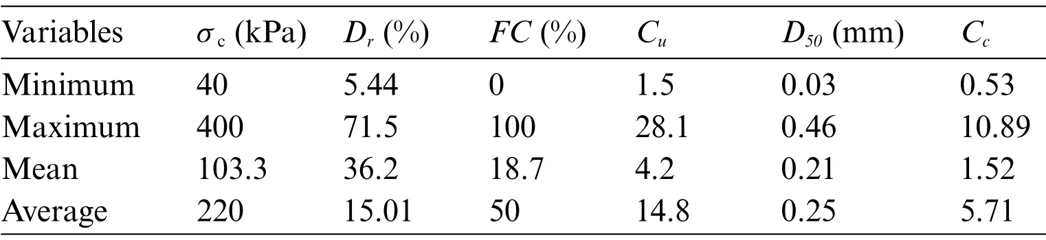
Table 1: Statistics of the entire input variables applied for the first ANN model

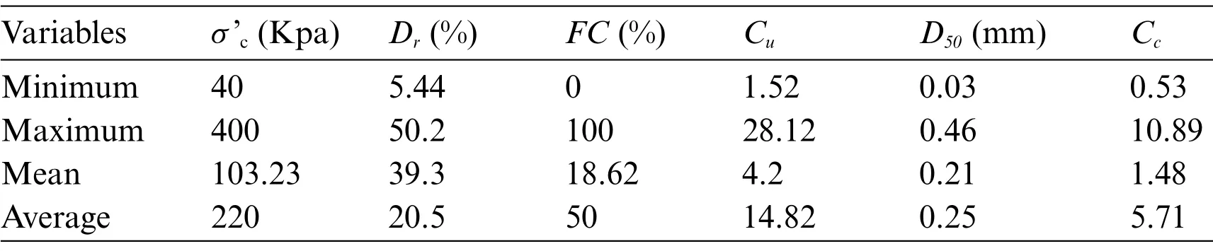
Table 2: Statistics of the entire input variables applied for the training phase of the first ANN model

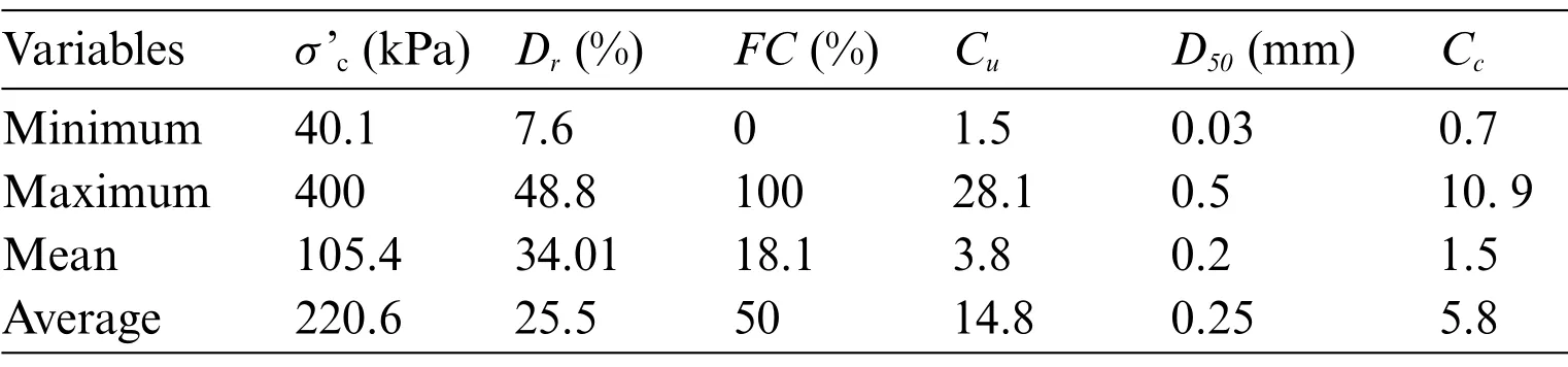
Table 3:Statistics of the entire input variables applied for the validating phase of the first ANN model

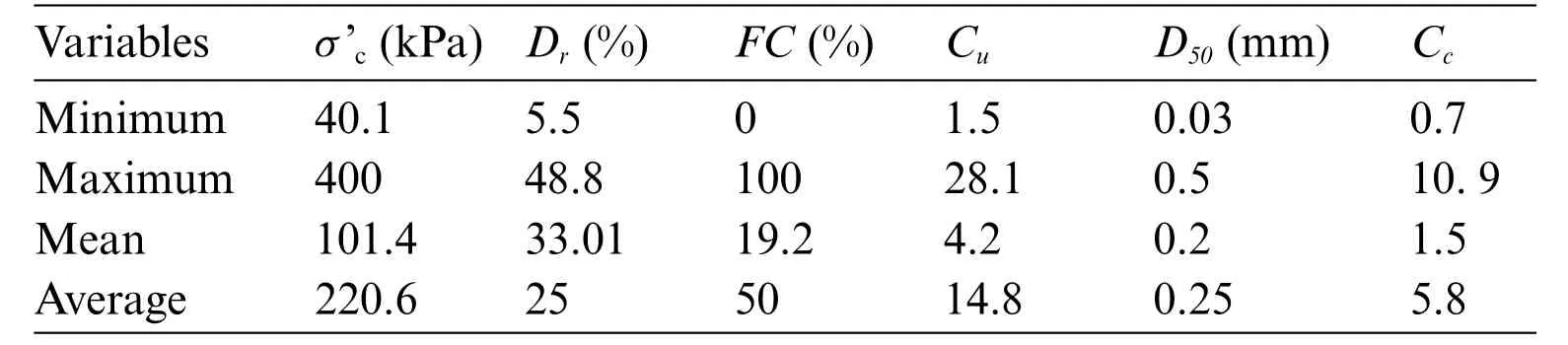
Table 4: Statistics of the entire input variables applied for the testing phase of the first ANN model

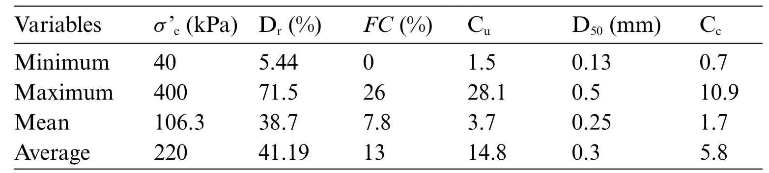
Table 6: Statistics of all input variables applied for the second ANN model

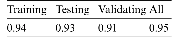
Table 5: Correlation coefficient of the first ANN model

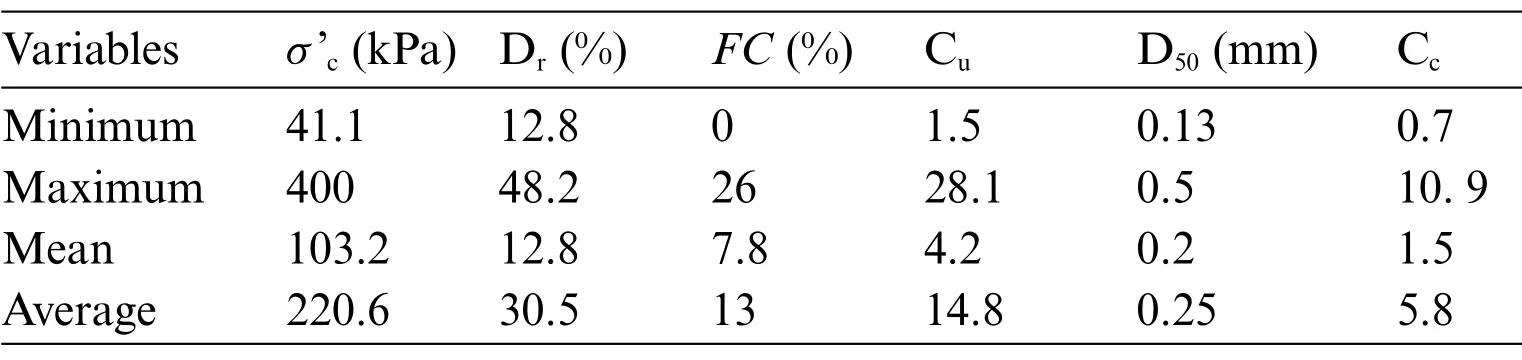
Table 7: Statistics of all input variables applied for the training phase of the second ANN model

Table 8: Statistics of the entire input variables applied for the validation phase of the second ANN model

Table 9: Statistics of all input variables applied for the testing phase of the second ANN model

This study investigates the effects of all parameters, includingCCwhile also paying special consideration to the influence ofFCin different range according to its critical value in seismic soil liquefaction assessment.To achieve this goal,two different ANN models,one using the entire dataset and the other using the samples withFCvalue of less than critical value,were developed to compare their predictions for validating and choosing the best one.In development of the models the validation phase was also performed to eliminate overtraining of the models.The data division was performed considering statistics characteristics of the variables instead of performing randomly to increase the accuracy of the trained models.Furthermore, to the best of the author’s knowledge, there has been no previous due attention to the uncertainties of parameters to predictW,which was the motivation behind performing the sensitivity analysis via MCS simulation to investigate the effect of uncertainty and the mean value of parameters on liquefaction resistance.Because of the numerous samples required by MCS and the relative data scarcity,in this study,the MC simulation was performed based on an ANN model developed in this study.

2 Methods Based on Laboratory test Results

Figueroa et al.[75] developed two equations to evaluate unit energy (E) in a cyclic triaxial test.Alkhatib[76]introduced ER to measure liquefaction resistance.ER is a ratio of the energy computed by area under the stress-strain hysteresis loop to the initial effective confining stress, and through conducting laboratory cyclic triaxial tests.The presented model is as below.

Extensive research has been performed at Case Western Reserve University on energy-based evaluation of liquefaction [31,38–41,75,77–79].In all procedures,Wuwhich is the area of the stressstrain hysteresis loops up to the initial liquefaction point was used to define liquefaction resistance.Parameter ofδWwas introduced first time by Figueroa et al.[31,75,77].They conducted 27 torsional shear tests on a Reid Bedford sand sample at different shear strain amplitudes and confining pressures and developed a model.

Liang et al.[13,41]conducted 74 liquefaction torsional shear tests on Reid Bedford sand,Lower San Fernando Dam (LSFD) silty sand, and Lapis Luster Dried sand (LSI-30) through random loading.From the test results, they performed a regression analysis and presented an equation to estimateδW.

Kusky [78] developed two equations according to 27 strain-controlled torsional triaxial tests,which were conducted on samples of Reid Bedford.

Rokoff[79]conducted some cyclic torsional shear tests on Nevada sand to investigate the influence of particle size distribution onδW.The regression was limited to special soil properties and geology related to the samples of Nevada region,which containsCuandCcas below:

In addition,Figueroa et al.[40]confirmed thatCuandCcaffectδWmore thanandDr.Wallin[80] presented three equations for Nevada sand, LSFD silty sand, and Reid Bedford sand through statistical analysis of tests results which were conducted by other researchers[39,75].

Baziar et al.[35]collected a large dataset from performed shear,cyclic triaxial,and torsional shear laboratory test results,which contained 284 samples from the literature.They developed two Artificial neural network (ANN) models to obtain a correlation between input parameters and Log (W).The first developed ANN model contained six input parameters (σ’c,Dr%,FC%,Cu,D50,Cc) while the second model was developed by eliminating the parameterCc.They subsequently demonstrated thatFChas the highest effect onWby carrying out a sensitivity analysis.By adding a new dataset to Baziar et al.[35]with the same parameters and applying multigene Genetic Programming,Baziar et al.[45]developed an equation to measureWand then used case histories earthquake data plus laboratory test data to validate and present the accuracy of their model.They concluded that the value ofWhas a complicated relationship withFC.Alavi et al.[46]presented three equations to estimate Log(W)through applying MEP,GP,and MEP and with the same database and parameters as Baziar et al.[35],as mentioned in the appandix and Table A1.In addition,they conducted sensitivity analysis and confirmed thatWis more affected byDrandσ’cthan other parameters.Zhang et al.[38]collected 302 samples for their database, which contained six cyclic simple shear, 18 centrifuges, six cyclic simple shear, and 217 cyclic tests.They developed a MARS model with the same five input parameters with Cavallaro et al.[10] to evaluate Log (W).They validated their model using 22 centrifuge test results conducted by Dief[81].

3 Methodology

3.1 Artificial Neural Network

Artificial Neural Network (ANN) is defined as brain model systems, which are collections of mathematical models containing cells (here called neurons) interconnected by links.The goal of ANN is to utilize a training process to learn a nonlinear multiplex relation between parameters to approximate a target (output).Training is the process of calculating weights, which indicates the strength of the links between neurons.There are several neural network types proposed, but feed forward neural networks are the most capable and commonly applied type.Among all classes of neural network topologies, Hornik et al.[82] demonstrated multilayer perceptrons (MLP), which are supervised networks, with the best capacity and ability to approximate any function with high accuracy.These include three types of layers: an input layer which distributes the input data and contains one neuron for each input variable, one or more hidden layers which perform non-linear transformations,additions,and multiplications;and an output layer for estimated final results,which contains a number of neurons equal number of targets meant to be approximated by the ANN model.The backpropagation algorithm is one of the most commonly used algorithms for training ANN’s.Here, connection weights are updated by estimating error and distributing it through the layers of neurons.It contains two steps that are iterated to obtain a pre-specified tolerance range of the output.In the first step, the network generates an output, and in the second step, the estimated error at the output layer is distributed to the hidden layers and then to the input layer to modify the weights.Each neuron’s error is calculated by:

Further,the overall neurons’output is estimated by:

The correlation coefficient(R)is the most common and capable tool to test the performance on networks given by:

Network samples are commonly separated into two subsets randomly;the first one is the training set to train the network by adjusting the weights of the network, and the second one is the testing set.Testing samples are not used in the training step and are applied to assess the performance of the trained network.A new sample set, called validation set, should be selected to prevent overtraining the network which occurs when the accuracy and the correlation coefficient increase,but the accuracy and the correlation coefficient of the validation samples set decreases.When overfitting starts,training should be stopped.

3.2 Monte Carlo Simulation and Uncertainties

The Monte Carlo method was introduced first during research on the atomic bomb in the beginning of the 1940s.The main idea is using random samples of inputs or parameters to discover the response of a complex process or system through observing the fraction of numbers.It involves three main steps:

1.Generating random input samples called scenarios.

2.Simulating each scenario to explore the response.

3.Evaluating outputs of all simulations to estimate statistics certificates and properties such as minimum and maximum values,mean value,and distribution function for each variable.

Conservative values of loads and soil properties cannot be reliably assumed due to inaccuracy in measurements and models, as well as the inherent variability in the systems under consideration.In geotechnical soil properties, these uncertainties are categorized into two groups: aleatory and epistemic [83].Aleatory uncertainties are defined as natural randomness such as spatial variability of soil properties and are related to inherent randomness, which cannot be reduced by adding new data and information.Epistemic uncertainties on the other hand, are caused by a shortage of data,information,and measurement procedures or model error as well as non-standard equipment,laboratory instruments,and random testing effects[84].Reliability approaches provide a formal way to deal with uncertainties and quantify them.Monte Carlo Simulation(MCS)conducts risk assessment by providing a probability distribution for any variables due to their uncertainties to estimate the possible outcomes of an uncertain phenomenon.

3.3 MCS Based ANNs Response Surface for Sensitivity Analysis

The main idea of the response surface method is a computational calculation reduction.In the classic form,the surface was approximated through an equivalent function such as polynomial form[85],which is not capable of modeling high nonlinear phenomena[86]such as liquefaction.Thus,in this study,the response surface which belongs to the ANN trained model is applied.The procedure of MCS-based ANNs response surface for sensitivity analysis is described in the flowchart of Fig.1.

Figure 1:Flowchart of the procedure proposed for performing sensitivity analysis

4 Models Presented in this Study

4.1 Databases and ANN Models

In this study,two different databases were arranged to train two ANN models to investigate the complex influence ofFCon liquefaction resistance.According to previous research[23,27,29–34,36–39,41],six parameters of(kPa),Dr (%),FC(%),Cu,D50(mm),andCcwere assigned as the inputs to create ANN models to calculate Log (W) as a target.The first dataset includes 284 experiments created by Baziar et al.[45],including 217 cyclic triaxial laboratory test results[87],six laboratory cyclic simple shear experiments[87]and 61 cyclic torsional laboratory tests[39,86]in addition to 22 samples added from Verification of Liquefaction Analyses by Centrifuge Studies (VELACS) [44,79,88], 48 cyclic trixial laboratory test results[89],20 laboratory test results from Dief[81]and 27 cyclic torsional laboratory test results [44].Overall, the main dataset was created, including these 403 samples, and divided into three groups according to the statistical factors.Of all,approximately 15%of the samples(60 samples)were considered for the testing phase,the same sample numbers for the validating phase,and an extra 283 samples for the training of the model.Despite the random division, the division of samples was performed while considering statistical factors of samples to achieve more accurate models compared to simple random allocation.Therefore, all three groups provided with similar statistical properties,as reported in Tables 1–4.For example,in the first dataset,the mean value ofFCin the entire dataset,training group,validating group,and testing group were 18.7,18.62,18.1 and 19.2,respectively.The same construction ANN of MLP with one hidden layer with the previous research[35]were applied to focus and demonstrate the positive influence ofFCvalue consideration and applying the validating phase as well as data division according to statistical factors.The characteristics of the first ANN model are presented in Table 5 with anRvalues higher than 90%,which defines the high accuracy of the ANN model to predict the target of logW.

Tao[44]studied the effect ofFCvalue on the liquefaction resistance by considering the void ratio.He demonstrated thatDrbecomes more effective when theFCgrows above 28%.He declared that there is no clear correlation between the entire range ofFCand liquefaction resistance.Therefore,in this study,the second database was arranged by collecting just samples withFCvalue lower than 28%to train an ANN model and hence samples withFChigher than 28%were eliminated from the dataset.Consequently,the second dataset contains 309 samples,which were divided into three parts,considering to have similar statistics certificates to achieve a more capable and accurate model.Around 15%of samples(44 samples)were selected for testing,equal portion and numbers for validation,and 221 samples for training the model.The characteristics and statistical factors of the second database are summarized in Tables 6–9.For example,the mean value ofFCin all datasets(including training group, validation group, and testing group) were 7.8, 7.9 and 8.1, respectively.Note that because of deleting 94 samples includedFCvalue of larger than 28%,the second dataset and its subsets would provide different statistical factors than the first dataset.The characteristics of the second ANN model are presented in Table 10.It can be seen that the value of R for all groups in dataset division(i.e.,all data,training data,validating data,and testing data)is greater than 90%,which indicates a high power fitting model.

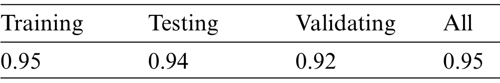
Table 10: Correlation coefficient of the second ANN model

4.2 Comparison of the Predicted Value of W Using the ANN Models and Available Models

In this section, the results of the ANN models are compared to the other four well-established models i.e., GP, LGP, MEP and MARS [38,46] to evaluate their capability.For more details about these models,refer to the Appendix.

To achieve this goal, 20 laboratory test results from Dief [81], performed on Nevada sand and Reid Bedford sand,considering the range of applied database are selected.Note that these 20 samples were not used in the database to construct the two ANN models developed in this study.The results predicted by these four models and two presented ANN models are presented in Table 11.

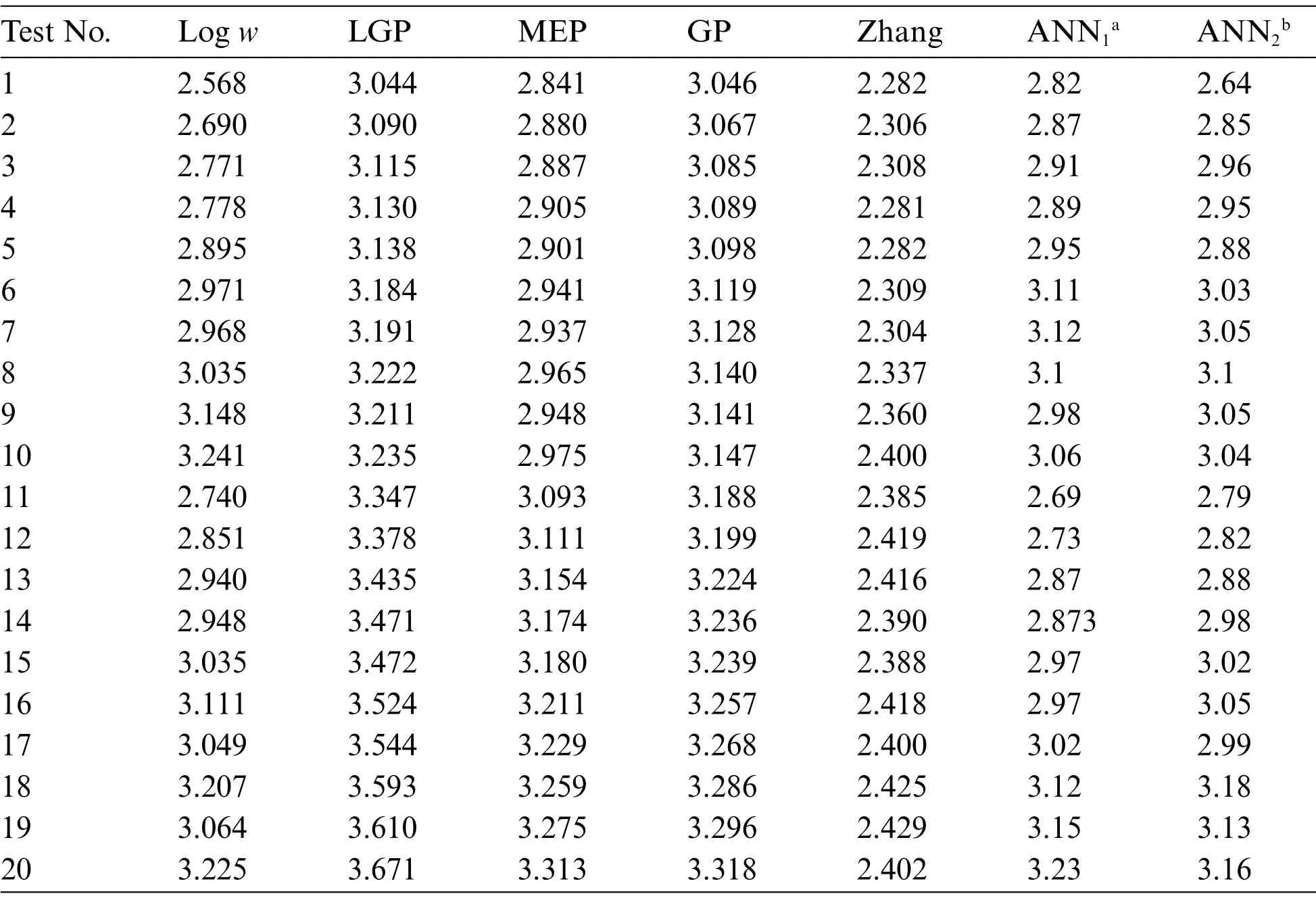
Table 11:Results predicted by two presented ANN models,four available models and measured values of 20 samples

To compare the capability and accuracy of all six models,three criteria of root mean square error(RMSE),mean absolute error(MAE),and R2are estimated and summarized in Table 12.As can be seen,two ANN models show higher agreement and less error between predicted and measured results in comparison with other available models.

Fig.2 illustrates that all predicted values through ANN models are close to the measured values for log(W).Two ANN models developed in this study predict log(W)with high accuracy,as presented in Table 12.The first and second ANN models predicted log(W)with R2of 0.77 and 0.83,respectively that are higher than the value of extra four models.In addition,the first ANN with RMSE and MAE values of 0.13 and 0.11,respectively,and the second ANN(referred to as ANN28 herein)with RMSE and MAE values of 0.1 and 0.09,respectively,demonstrate the highest precision.

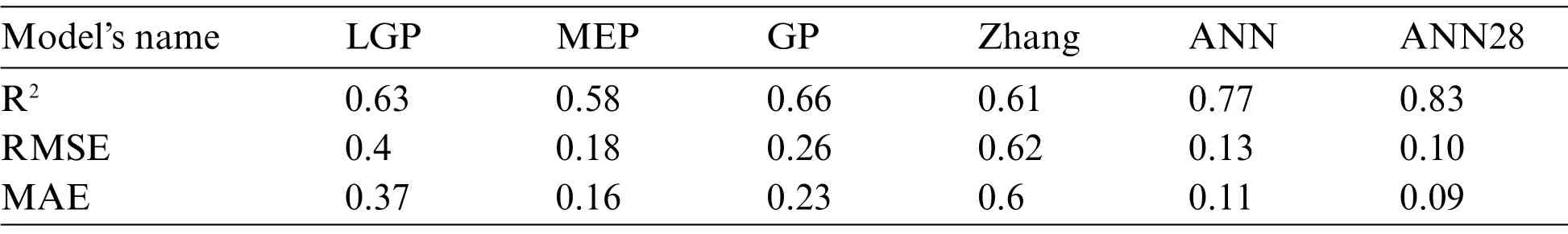
Table 12: Summary of comparison between two presented ANN models and four additional models

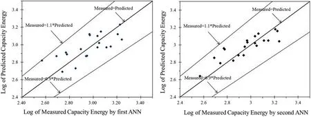
Figure 2:Capacity energy predicted by ANN models vs.measured values of laboratory tests

Based on the illustrated figures and Table 12,the two presented ANN models are the most accurate and capable models for predicting log (W) and between them, the second model, which contains a dataset with a limitedFCvalue of less than 28%,indicates more accuracy.Note that the ANN28 model was developed based on fewer samples due to eliminating samples withFCvalues larger than 28%.

4.3 Sensitivity Analysis

As mentioned in Section 4,most geotechnical parameters,soil properties,and applied loads are uncertain.To deal with these uncertainties,reliability methods have been used to quantify and capture these uncertainties.In this study, MC simulation was applied to perform sensitivity analysis and investigate the influence of parameters and their uncertainties by changing their mean values and coefficient of variations (COV) or standard deviation (ν).Monte Carlo simulation requires a large number of samples to present a reliable response.Providing such a large number of samples is costly and time-consuming.Therefore, to overcome this shortage, the second ANN model was applied to provide a response surface for MCS to be able to conduct sensitivity analysis.Phoon et al.[84]suggested a mean COV of 19%for sand withDrranging from 11%to 36%;Therefore,in this study to evaluate this parameter’s effect on log(W),it was supposed to have a mean COV equal to 20%with minimum and maximum value of 10%and 30%,respectively.Subsequently,was suggested to have COV equal to 10%[90]to inspect the effect of its uncertainty,where the maximum and minimum COV values were assumed to be 5%and 15%.

Furthermore, given the fact that with a small value ofν, the distribution function supposition error is insignificant,normal distribution was assigned to all variables[90,91].All statistical properties of parameters are summarized in Tables 13 and 14.It should be mentioned that during parametric sensitivity analysis of each variable,the other five variables fixed in their mean value and mean COV value,without changing,then analysis was conducted.

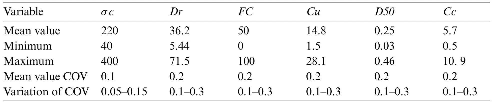
Table 13: Statistics of the first ANN model’s variables

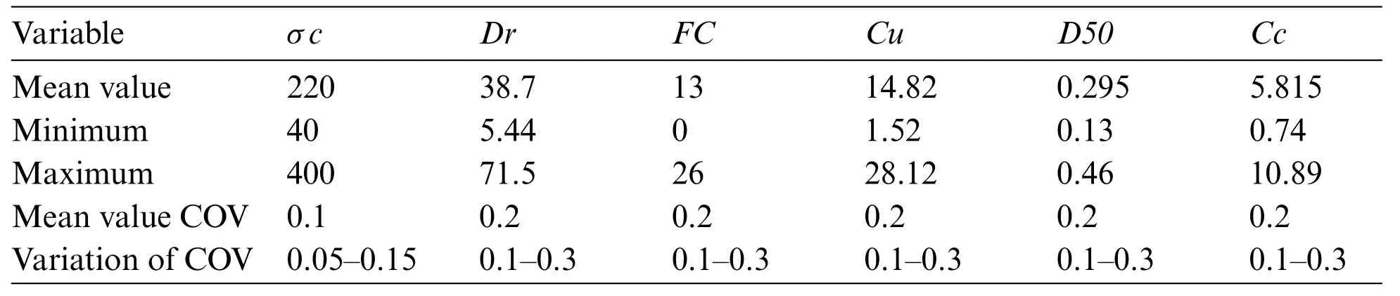
Table 14: Statistics of the second ANN model’s variables

Additionally, in order to conduct a sensitivity analysis through MC simulation, a definition of correlation coefficient(ρ)is required.By considering the independency of all six input parameters,ρamong all parameters is supposed to be 0.The value of 2.9 was chosen for reliability analysis to assess the cumulative probability density function.As can be observed in Fig.3,the probability of log(W)larger than 2.9 is illustrated as a function of the parameters and their uncertainties.

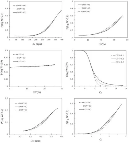
Figure 3:The parameters vs.probability of logarithm of capacity energy greater than 2.9

By considering Fig.3,which plots parametersvs.probability of if log(W)be higher than 2.9,can be seen, there is a slight increase (i.e., 15%) in log (W)＞2.9 is observed forσ’cfrom 44 to 250 and then,it grows dramatically to 75%atσ’cbeyond 250.Upon increasing COV from 5%to 10%and then 15%,probability grows two times by 1.5%.The probability rises slightly from 4%to 60%in the range ofDrfrom 5.44 onwards.It experiences an impressive rise to 60% asDrincreases to 71.5% also, by growing uncertainty as COV from 0.1 to 0.2, and then 0.3 in the critical range ofDrbetween 35%to 70%, the probability shows two increases of 3%.During the growth of theFCvalue until 28%,the probability shows slight growth from 21%to approximately 24.5%and it experiences a negligible increase while the COV changes.Furthermore, the probability of log (W)＞2.9 illustrates a falling range from 100%to 0%during the range ofCuin this study.Next to that,by increasing COV from 0.1 to 0.2,and subsequently 0.3 in the critical values between 13 to 16,the probability augments around 7%every time.There was a steady climb of around 19%in the probability in the range of theD50in this study.In addition,by increasing any 0.1 in COV,from 0.1 to 0.2 and then 0.3,the probability rises negligibly less than 1% for log (W)＞2.9.Whereas, by any 10% increase in COV ofCcresults show around 2.5%growth in the probability in a sense that the probability goes up around 58%in the range ofCcfrom 0.74 to 10.89.

5 Summary

In this study,ANN was used to develop models to estimate the liquefaction resistance of sandy soil based on the capacity strain energy concept and using laboratory test data.The validating phase was performed,in addition to the testing and training phase,to avoid overtraining the model and increasing the model’s capability.An extensive database was collected from literature,including triaxial,simple shear,torsional,and centrifuge test results.ANNs are powerful tools for developing models that can take into account the complexity and non-linearity of the liquefaction issue.To inspect the complicated influence ofFCon liquefaction resistance of soil, according to research results presented by Tao[44], two ANN models were developed.The first model was developed using a complete dataset,while the second one was based on the samples byFCless than 28%.The accuracy and capability of the presented models were demonstrated by comparing their predicted values for log(W)with four other available well-known equations.To conduct this comparison, 20 liquefaction test results from Nevada sand and Reid Bedford sand [41], which were independent of the two applied datasets for training the models,were considered.Finally,to investigate the effect of uncertainty in geotechnical parameters,a sensitivity analysis was performed using MCS based on the response surface provided by the second presented ANN model,which showed higher accuracy.The results of sensitivity analysis were illustrated through some graphs to indicate the correlation between the variables and their uncertainties with the liquefaction resistance of the soil in order to capacity energy.The limitation of the present study includes its application in the issue of strain energy,not in the other methods such as stress-based or numerical methods.

6 Conclusions

In conclusion,this study has demonstrated:

1.Artificial neural network(ANN)is a powerful tool to assess liquefaction in soil with high nonlinearity.Adding validation phase and performing data division by considering the statistical aspects,instead of random division,provides significant precision on the model.

2.The second ANN model(considering samples withFCless than 28%)is able to predict log(W)with higher accuracy.As it includes a smaller number of samples in the dataset in comparison with the first ANN model,it is evident that differentFCvalues provide a different effect on liquefaction resistance.

3.The parameter ofCcsignificantly affectedWand should be considered to predict theWvalue.

4.The uncertainty of parameters had a considerable impact on liquefaction resistance.As a result,performing probabilistic frameworks and models are suggested by the authors instead of deterministic models to consider and quantitate these uncertainties’effects.

Funding Statement:This work is supported by the Scientific Innovation Group for Youths of Sichuan Province under Grant No.2019JDTD0017.

Conflicts of Interest:The authors declare that they have no conflicts of interest to report regarding the present study.

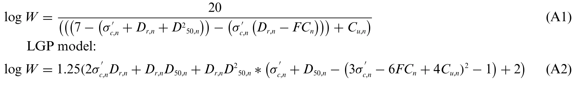
Appendix

Alavi et al.[46] developed three equations using genetic programming (GP), linear genetic programming (LGP), and multi expression programming (MEP) to evaluate the strength of soil liquefaction according to the capacity energy as below:

GP model:

MEP model:

The normalized variables used in these three equations are defined as below:

Zhang et al.[38]developed an equation using MARS as below:

Table A1 presents all the coefficients required in Eq.(A5).

Table A1: Coefficient of Eq.(A5)