Comparison of differential evolution,particle swarm optimization,quantum-behaved particle swarm optimization,and quantum evolutionary algorithm for preparation of quantum states

Xin Cheng(程鑫) Xiu-Juan Lu(鲁秀娟) Ya-Nan Liu(刘亚楠) and Sen Kuang(匡森)

1Department of Automation,University of Science and Technology of China,Hefei 230027,China

2Department of Mechanical Engineering,The University of Hong Kong,Hong Kong 999077,China

3Quantum Machines Unit,Okinawa Institute of Science and Technology Graduate University,Okinawa 904-0495,Japan

Keywords: quantum control,state preparation,intelligent optimization algorithm

1.Introduction

One goal of quantum control is to guide the dynamics of a quantum system to a desired quantum state or achieve some specific operations,[1,2]which plays an important role in many quantum applications, for example, NMR,[3,4]femtosecond laser,[5]superconducting qubits,[6]and the preparation of quantum gates in quantum computing.[7]Scientists and engineers have developed a variety of methods for the preparation of quantum states, e.g., optimal control,[1]adiabatic control,[8]feedback control,[9]robust control,[10]learning control,[11]and Lyapunov control.[12]Among these methods,learning control has strong application prospects for complex quantum control problems and has been successfully applied to many practical control problems.[6,13-15]In general,learning control can be divided into two categories: gradientbased and gradient-free.The well-known GRAPE and Krotov algorithms belong to gradient-based learning algorithms,which were widely used in numerical simulations and actual experiments.[3,16,17]However, for some complex control problems, it is difficult to obtain the gradient information of a system.In addition, some systems may have local optimal points.[18]In this case, the gradient algorithm is difficult to achieve the control objective.A natural idea to solve such problems is to use random search methods to find optimal control laws.This corresponds to another type of learning methods, i.e., gradient-free intelligent optimization algorithms, including genetic algorithm (GA),[19]particle swarm optimization(PSO),[20]differential evolution(DE),[21]etc.At present, intelligent optimization algorithms have been widely used in quantum physics.For example,GA had been successfully implemented in the control of molecular systems.[11]DE was used for identifying the unknown parameters for different chaotic systems.[22]Donget al.[13,14]proposed an improved DE algorithm to solve the robust quantum control problem.In Refs.[6,15],a direction averaged DE and a subspace-selective self-adaptive DE had been used to find the control pulses for high-fidelity quantum gates respectively.Reference[23]used the PSO combining with the path planning method to determine the unknown parameters in the control laws and realized the high-fidelity transfer to target eigenstates of highdimensional quantum systems.

Existing studies have shown that PSO and DE have significant advantages over other traditional intelligent optimization algorithms.[24]Based on quantum mechanisms,quantum versions of intelligent optimization algorithms have been developed,e.g.,quantum evolutionary algorithm(QEA)[25]and quantum-behaved particle swarm optimization (QPSO).[26]The QEA is a probabilistic optimization method based on quantum computing.It uses qubit encoding to represent chromosomes and quantum-gate updates to complete evolutionary search.The QPSO was invented by incorporating the particle behavior in quantum mechanics and the traditional PSO algorithm.For some problems in other areas,QEA and QPSO are superior to GA and PSO.[27,28]However, they are rarely used in the field of quantum control.Although Zahedinejadet al.[29]compared the gradient algorithms and the intelligent optimization algorithms for the preparation of high-fidelity quantum gates, they only considered the traditional DE and PSO.A natural question occurs,that is,do quantum versions of intelligent optimization algorithms perform better with respect to their traditional versions for quantum control problems? In this paper, we will answer this problem and try to provide a valuable reference for the choice of intelligent optimization algorithms solving actual quantum control problems in the future.

In this paper, we use four intelligent optimization algorithms,i.e.,DE,PSO,QPSO,and QEA,to find control pulses to achieve the state preparation of closed and open quantum systems.The contributions of this paper are as follows.First,the control performance of the four algorithms is compared and their differences are analyzed.Second, we consider and compare the robustness of the control pulses found by the four algorithms for the perturbed quantum systems.Third,by comparison,a new conclusion is obtained: the QPSO has best performance among the four intelligent optimization algorithms and is almost optimal for all considered performance criteria.This provides an important reference for the future use of intelligent optimization algorithms in solving complex quantum control problems, i.e., the QPSO based on quantum mechanisms is a powerful candidate.

The rest of this paper is organized as follows.Section 2 describes the general closed and open quantum control problems.Section 3 presents the rules of numerical simulation.Numerical simulation results under both undisturbed and disturbed conditions are provided in Section 4.Concluding remarks are given in Section 5.

2.Control problem description

In quantum control,one usually decomposes the Hamiltonian of a system into a controllable and an uncontrollable parts and steers the dynamics towards a desired evolution through varying the controllable part.[29]

2.1.Closed quantum systems

A quantum system that has no or negligible interactions with the external environment is called a closed quantum system.And for a generalN-dimensional closed quantum system,its state evolution obeys the following Schr¨odinger equation:

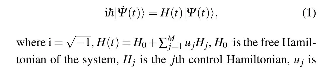
For theN-dimensional closed system in Eq.(1),the quantum state preparation problem can be stated as follows.Within a given timeT, find suitable controlsuj(j=1,2,...,M) to drive the system to a desired target state|Ψf〉from a given initial state|Ψ0〉with the highest fidelity possible.To this end,we define fidelity as

where|Ψ(T)〉is the state of the system at timeT.Thus, the problem of preparing the target state|Ψf〉can be expressed as an optimization problem,that is,

s.t.

2.2.Open quantum systems

A quantum system that has non-negligible interactions with the external environment is called an open quantum system.Its dynamic evolution is no longer consistent with the unitary evolution,because the interaction with the external environment causes decoherence.Therefore,the state of the system cannot be described by the state vector|Ψ〉in Eq.(1),but by the density matrixρ.TheN-dimensional open quantum system’s dynamic evolution can be described by the Lindblad master equation as[30]

where the non-negative coefficientsγkspecify the relevant relaxation rates of thekth channel(in this paper, we set it asγk=1),Lkare appropriate Lindblad operators,and

The first term on the right side of the equal sign of Eq.(4)represents the Schr¨odinger term, and the second term is the dissipation term,which represents the decoherence effect caused by the interaction between the system and the environment.When the dissipation term is 0, Eq.(4) can be regarded as the dynamic evolution equation of the closed quantum system,which is equivalent to Eq.(1).The derivation from the evolution equation (1) of the closed system to the evolution equation(4)of the open quantum system is referred to Ref.[30].

For the open system(4),we define a coherence vector asx:=(x1,x2,x3,...,xm)T=(tr(U1ρ),tr(U2ρ),...,tr(Umρ))T,

where iU1,iU2,...,iUm(m=N2-1) are a set of orthogonal generators of the special unitary groupSU(N).Thus, the density matrix can be written as[31]

By substituting Eq.(6) into Eq.(4), the open quantum system (4) can be expressed as the following coherence vector equation:

where the superoperators LH0,LD,and LHj(j=1,2,...,M)are(N2-1)×(N2-1)square matrices,andl0is an(N2-1)-dimensional column vector.Their specific forms are[31,32]

where (·)strepresents the element of thesth row and thetth column of a matrix, and Tr(·) is the trace of a matrix.The fidelity is defined as[32]

where||·|| is a vector norm,xfis the coherence vector of the target state andx(T)is that of the system state at timeT.Similarly, the control task can be described as the following optimization problem:

s.t.

3.Comparison backgrounds

In this section, we list several backgrounds for the comparison of the four algorithms.

1) Control fields We adopt piecewise constant controls forujin Eqs.(1) and (4), that is, we discretize the time interval [0,T] intoDequal time segments, where the length of each segment isδt=T/Dand the controlujtakes a constant in each segment.Thus, our control task is to find a suitable pulse sequenceu(1),u(2),u(3),...,u(D)on[0,δt),[δt,2δt),..., [(D-1)δt,Dδt] to drive the system to the desired target state.In this paper,we takeT=4 a.u.andD=100.

2)Control amplitudes In practical applications,the amplitude ofujis usually bounded, that is,uj(k)∈[umin,umax].In this paper,we assume thatumax=10 andumin=-10.

3) Hyperparameters For the parameters in each algorithm,we set their values as follows.

DE:The scaling factor isF=0.5 and the crossover factor isCR=0.3.PSO:The two learning factors arec1=1 andc2=1.QPSO:The contraction-expansion coefficientα=0.5.QEA: The quantum gate updating rule is provided in Ref.[25].

4)Evaluation criteria In this paper, the fidelity will be our performance indicator.The process of intelligent optimization algorithm starts from an initial population and seeks the optimal solution of the optimization problem through continuous iteration.Therefore,in order to ensure fairness in the algorithm evaluation process,we take the following measures:1) the initial population size of the four algorithms remains the same, which is 100; 2) considering that each algorithm needs to randomly generate initial solutions, we repeat each algorithm 10 times (10 episodes) to reduce the effect of randomness, and the best, mean and worst fidelities of the 10 episodes will be used to measure the performance of the algorithms, where the mean fidelity that best characterizes the actual performance of the algorithms will be prioritized; 3)for each episode, the termination conditions of the four algorithms are also the same, that is, the number of iterations reaches 10000.

5)Data availability Please refer to the Appendix for the details of the data of the system models in numerical simulations.

6) Numerical simulation platform The computer configuration is intel(R)Core(TM)i9-10900KF CPU@3.7 GHz,RAM 64 GB, Windows 10, MATLAB 9.9.0.1467703(R2020b).

4.Comparison of algorithms

For the problem of quantum state preparation discussed in Section 2,we conduct numerical simulations on two-level,three-level and four-level quantum systems under both undisturbed and disturbed conditions,and at the same time compare the performance of the four algorithms presented in this paper.

4.1.Results and analysis

In this section,several closed and open systems are considered in simulations.The simulation results are shown in Table 1 and Fig.1, where Table 1 presents three types of fidelities (i.e.,Fbest,Fmean, andFworst) for the four algorithms and six quantum system models and Fig.1 describes how the mean fidelity of 10 episodes changes with the iteration number.

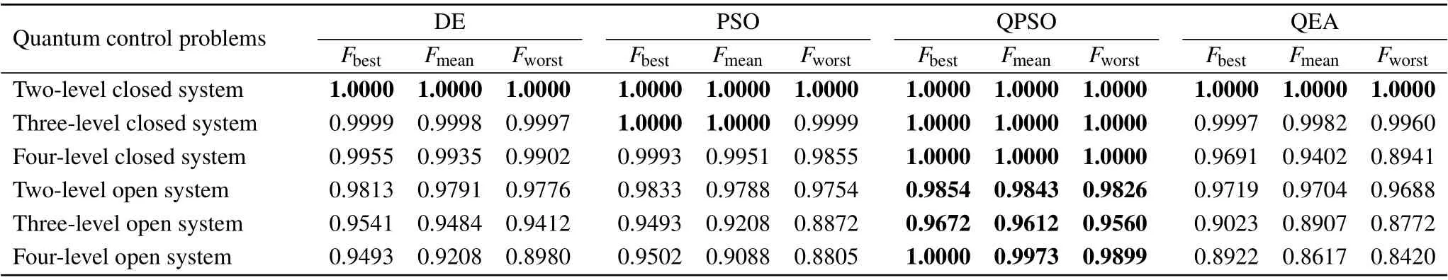
Table 1.The simulation results of the four algorithms without disturbances,where each algorithm runs 10 episodes with Fbest,Fmean,and Fworst being the best,mean,and worst fidelities of 10 episodes,respectively.The optimal values are in bold and the data greater than 0.99995 are regarded as 1.

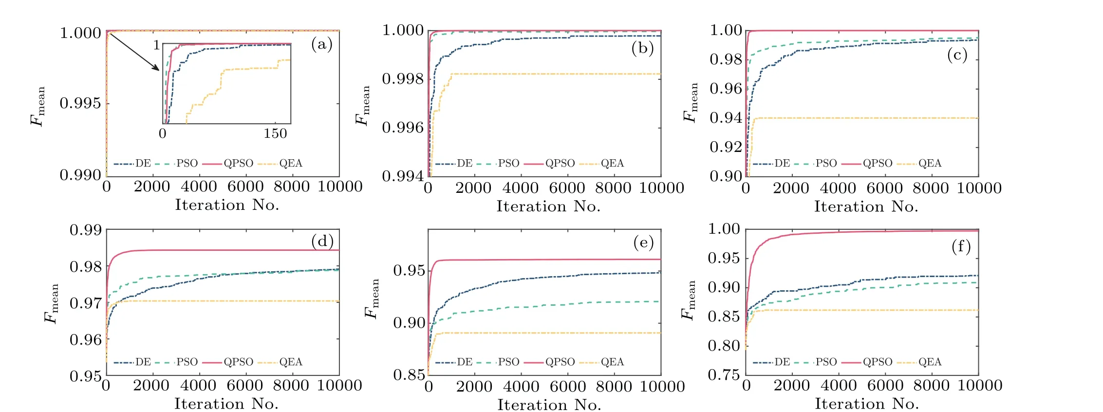
Fig.1.Quantum state preparation of six quantum systems: Fmean vs.iteration No.of the four algorithms.The Fmean here refers to the mean fidelity of the algorithm running 10 episodes.(a) Two-level closed quantum system; (b) three-level closed quantum system; (c) four-level closed quantum system;(d)two-level open quantum system;(e)three-level open quantum system;(f)four-level open quantum system.

From Table 1, we can clearly obtain the following three conclusions.First,for the problem of state preparation of both closed and open quantum systems, QPSO outperforms the other three algorithms in the best,mean and worst fidelities of 10 episodes.And the superior performance of QPSO is more obvious for open quantum systems.For example,the mean fidelity of QPSO under 10 episodes is 0.9973 for the four-level open quantum system,which is 8.3%,9.7%and 15.7%higher than those of DE, PSO and QEA, respectively.Second, the performance of QEA is worst with respect to the other three algorithms in all the aspects except for the two-level closed system.Third,PSO has a slight advantage over DE for closed quantum systems and it is reversed for open quantum systems.

Figure 1 can also describe the characteristics of the four algorithms in the iterative process.Compared with the other three algorithms, QPSO can always achieve a best performance and converges at a fast rate,while QEA performs worst and stops converging after several iterations for all these six quantum systems.

One might ask why QEA is bad and QPSO is excellent.For the QEA with the quantum gate update mechanism, a quantum gate is used to update the position of each particle.The rotation angle of the quantum gate is determined by a simple look-up table, which leads to the discontinuity of the updated value of each rotation and makes the update insufficient.On the other hand, the QEA is easy to fall into local optimums and therefore performs poorly in the quantum control problem.The superiority of the QPSO algorithm can be explained from its essential features.First,a particle described by a probability density function can appear in any region of the entire feasible search space with a certain probability.This enables each particle not to be restricted by velocity and therefore can converge faster.Second, in the iterative process, the average best position is introduced to assisting in updating the position of each particle,which can avoid all particles moving toward the present optimal value.Thus, the algorithm is not easy to fall into local optimal values,which actually improves the global search ability.Moreover, compared with the other three algorithms,the number of parameters of QPSO is least,which can improve the efficiency of adjusting the algorithm parameters.

According to the simulation results, QPSO is the best while QEA is the worst for the state preparation of closed and open quantum systems without disturbances.This provides us with an important reference when using intelligent optimization algorithms to solve some quantum control problems,i.e.,QPSO should be given a high priority.

4.2.Robustness

In this section,we consider the robustness of the four algorithms in the presence of disturbances.For an actual quantum system,there are always some external disturbances,inaccurate models,and errors in the control field.Here,we assume that the Hamiltonian of the systems in Eqs.(1)and(4)has the following form:[13]

whereΘ= (θ0,θ1,...,θM) andfm(θm) (m= 0,1,2,...,M)describes possible uncertainties.f0(θ0) represents the uncertainty of the free Hamiltonian,e.g.,the chemical shift in NMR.fm(θm) characterizes possible noises in the control fields or imprecise parameters in the dipole approximation.We assume thatfm(θm) are continuous functions ofθmand the parametersθmtakes values in[1-Em,1+Em],Em ∈[0,1].For simplicity, we also assume that all uncertain boundaries satisfyE0=···=Em=···=EM=E=0.2 andθmis equal to 1 in the absence of disturbance.

Based on the sampling learning method,we take the twolevel open system as an example to compare the robustness of the algorithms.For convenience, we setf0(θ0)=θ0andfm(θm)=θm.In the numerical simulation,we choose 9 training samples.Bothθ0andθmtake values of 0.8,1.0 and 1.2 in turn,thus forming 3×3=9 samples.

We first generate optimal control pulses for the four algorithms under 10 episodes by 9 trained samples as shown in Fig.2.To compare the robustness of the optimal pulses found by these four algorithms,we randomly selected 100 test samples for testing.Bothθ0andθmrandomly take 10 values in[0.8,1.2], thus forming 10×10=100 samples.The test results are presented in Fig.3.

Fig.2.The control pulses of the four algorithms learned by 9 training samples.

From Fig.3,we can see that QPSO is still a best choice,and the fidelities of all test samples are steady and high with respect to the other three algorithms,which shows that the control pulses trained by QPSO not only have best robustness but also have best control performance.The fidelities of DE in the test samples are more concentrated than those of PSO,that is,the trained control pulses are more robust.QEA still ranks bottom, the minimum fidelity of the test samples is nearly 0.92,lower than 0.98 corresponding to QPSO.And the fidelities of the test samples have large fluctuation range,which implies a poor robustness of control pulses.

Fig.3.The fidelity of 100 test samples under control pulses in Fig.2.

Figure 4 shows the effect of the fluctuations ofθ0andθmon the fidelities associated with the four algorithms.It is easily seen that the fidelity surface under the QEA is steepest in the parameter fluctuation space, which indicates a worst robustness.In contrast,the fidelity surface under QPSO is above those under the other three algorithms.Moreover,the fidelity surface under QPSO is relatively flat, which means that the corresponding control pulses have best robustness.

Fig.4.The robustness control landscape defined as the fidelity versus two uncertainty parameters under control pulses in Fig.2.

5.Conclusion

DE and PSO have been widely used in various quantum control problems.However, QPSO and QEA based on quantum mechanisms are rarely used in the field of quantum control.In this article, we used the four intelligent optimization algorithms(DE,PSO,QPSO,and QEA)to find control pulses to achieve the state preparation of closed and open quantum systems.The research in this paper shows that QPSO has best performances and QEA ranks bottom when disturbances are not considered.While for robust control problems with disturbances,QPSO still performs best and has obvious advantages over the other three algorithms.This provides an essential reference for the use of intelligent optimization algorithms solving complex quantum control problems, that is, QPSO is a powerful candidate.

Appendix A:Data for system models

Two-level closed quantum system model

Three-level open quantum system model

The three energy eigenstates of the three-level open quantum system are|1〉= (1,0,0)T,|2〉= (0,1,0)T,|3〉=(0,0,1)T.The Hamiltonian is

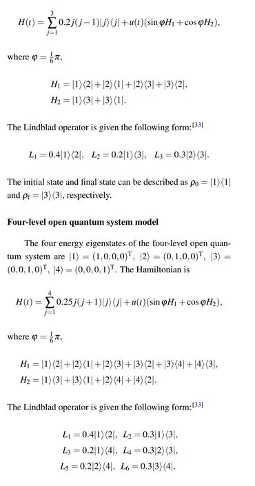
The initial state and final state can be described asρ0=|1〉〈1|andρf=|3〉〈3|,respectively.

Acknowledgement

Project supported by the National Natural Science Foundation of China(Grant No.61873251).