
A new method of constructing adversarial examples for quantum variational circuits
2023-09-05 08:47JingeYan颜金歌LiliYan闫丽丽andShibinZhang张仕斌
Chinese Physics B 2023年7期
关键词:丽丽
Jinge Yan(颜金歌), Lili Yan(闫丽丽),†, and Shibin Zhang(张仕斌)
1School of Cybersecurity,Chengdu University of Information Technology,Sichuan 610000,China
2Advanced Cryptography and System Security Key Laboratory of Sichuan Province,Sichuan 610000,China
Keywords: quantum variational circuit,adversarial examples,quantum machine learning,quantum circuit
1.Introduction
Quantum physics and machine learning are currently a focus of research, and based on these a new research field called quantum machine learning has been proposed.[1,2]Machine learning has developed rapidly over the past 20 years.It has solved many challenging problems and effectively promoted the development of artificial intelligence.[3–5]However,some machine learning algorithms are too complex to be implemented on classical computers in a reasonable time.[6]In addition, with the development of machine learning the network structure, parameters and algorithms of machine learning models are becoming larger and more complex.Generally, accurate models can only be trained with the support of a large number of data and calculations, which requires a lot of resources.Therefore, the development of machine learning is limited by the classical computer.Fortunately, the development of quantum computing has solved the above problems faced by machine learning.[7,8]Quantum computers can reduce the time required for large and complex machine learning algorithms.Quantum machine learning has achieved rapid progress in the past 10 years.Based on quantum properties such as quantum superposition, quantum entanglement and quantum measurement, many quantum machine learning algorithms have been proposed,[9,10]for example, Shor, Grover and HHL.[11,12]Quantum walks are another recent example.[13]Researchers have also designed some quantum machine learning algorithms based on classical machine learning algorithms,such as quantum support vector machine[14–16]and quantum principal component analysis.[17]Compared with classical algorithms,these algorithms achieve exponential acceleration.Quantum neural networks are an important branch of quantum machine learning.There are many kinds of quantum neural networks.[18–20]Most of them are constructed using quantum circuits, and the function of the neuron is replaced by quantum gates, with the angles of the quantum gates being the neural parameters.They take quantum states as input data, some take quantum states as output and some take the probabilities of measuring quantum bits as output.[21,22]Recently researchers have found that parameterized quantum circuits, i.e., quantum variational circuits, can be regarded as a kind of quantum neural network.[23]With the development of quantum hardware and corresponding software,quantum variational circuits will have broad application prospects.[24–27]
In classical machine learning it has been found that machine learning models are vulnerable.Adding a small and imperceptible perturbation to the input of a machine learning model may cause incorrect output of the model.In 2004,Dalviet al.found that linear classifiers are prone to errors in classification results caused by some carefully constructed perturbations.[28]Therefore, how to construct such perturbations and how to make the machine learning model highly robust against such perturbations have become new topics in machine learning research.This has given rise to the emerging field of adversarial machine learning.Szegedyet al.found an obvious example of perturbation in a deep learning environment for the first time, proving the vulnerability of machine learning.They took an image of a panda as the input of a machine learning model and added a small perturbation (imperceptible to the human eye)to it,and the model mistakenly identified it as a gibbon.[29–31]In quantum machine learning it has also been found that the quantum machine learning model is vulnerable to attack by a small imperceptible perturbation which makes the model output incorrect.[32]The example after the addition of a perturbation is called the adversarial example,and the key point in constructing adversarial examples is to obtain the gradient of the loss function with respect to featuresxof the examples.Siruiet al.obtained this gradient by an automatic differentiation method[33]in a classical computer,and they provide a thorough investigation of adversarial examples and attacks on quantum machine learning models.[34]
In this paper,we propose an innovative method to obtain the gradient,which is realized by quantum circuits in a quantum computer.Firstly, a series of quantum circuits are constructed according to the number of gradient components,and the measurement expectation of a qubit in each quantum circuit is obtained.Finally,the gradient is obtained according to the expectation.Analysis shows that this method is better than the existing automatic differential method and finite difference method.
2.Existing research
Suppose there is a trained quantum machine learning model;it is necessary to encodeNfeatures of normalized datax=(x1,x2,...,xN) into a quantum state|ϕ(x)〉=∑Ni=1xi|i〉by amplitude encoding,[35]taking|ϕ(x)〉as its input.Its loss functionL(|ϕ(x)〉,θ,y) is determined by its trained parametersθand the model inputxand labely.To construct a suitable adversarial example, we only need to search for a small perturbationδwithin an appropriate regionΔand add it to|ϕ(x)〉, which makes the value of loss function as large as possible so that the output of the model can deviate from the labely:
We add the perturbationδtoxthen the adversarial example
can be obtained.Specifically,the exact perturbationδcan be obtained by evaluating the gradient of the loss function with respect toxand multiplying it by a perturbation factorε;εdetermines the magnitude of perturbation
A quantum variational circuit can also be regarded as a quantum machine learning model,it consists of three parts:
(i)A prepared quantum state|ϕ(x)〉as its input.
(ii)A quantum circuitU(θ),which is parameterized by a set of free parametersθas its model.
(iii)Measurement of an observableMat the output as its output; this observable may be made up from local observables for each wire in the circuit, or just a subset of wires.It can be written as〈ϕ(x)|U(θ)†MU(θ)|ϕ(x)〉.
A simple example of a quantum variational circuit can be seen in Fig.1.It takes the expectation of a Pauli-Zbased measurement of just one wire as output and such a model can be a classifier.
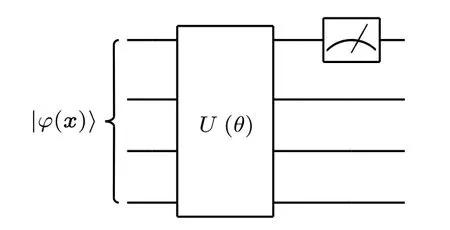
Fig.1.A simple example of quantum variational circuit.
To train such a quantum variational circuit, we need to evaluate the gradient of the loss function with respect to parametersθ,and the parameter-shift method[36]is usually used for this:
whereL(|ϕ(x)〉,θ,y) is the loss function,ϑis a single parameter of parametersθ,|ϕ(x)〉is the input andyis the label.We assume that the parameters of the quantum variational circuit have been trained well.To construct adversarial examples,we only need to define a perturbation factorε, then evaluate the gradients of the loss function with respect toxaccording to Eq.(3)to obtainδand then add it to|ϕ(x)〉to get the adversarial example|ϕ(x′)〉.Existing research[34]on evaluating the gradient of the loss function with respect toxuses the automatic differentiation method,[33]which is a method of calculating the gradient in classical computers by differentiating.
3.The proposed method
In this section,we propose a new method to evaluate the gradient of the loss function with respect toxfor quantum variational circuits and compare it with existing methods.
Suppose there is a trained quantum variational circuit.It takes|ϕ(x)〉 = ∑1xi|i〉 as input and the outputy′=〈ϕ(x)|U(θ)†MU(θ)|ϕ(x)〉, so its loss functionℒcan be written as
whereyis the label of the input datax.The gradient ofℒwith respect toxis ∇xℒ=(∂ℒ/∂x1,∂ℒ/∂x2,...,∂ℒ/∂xN), and each component of the vector is∂ℒ/∂xi=(y′−y)κi, wherei=1,2,...,Nandκiis
where|A〉=U(θ)∂|ϕ(x)〉/∂xiand|B〉=U(θ)|ϕ(x)〉.Obviously the key point to getting∂ℒ/∂xiis to obtainκi.Next,we will introduce a method to obtainκi.
Firstly,nqubits|0〉called the‘data register’and one|0〉called the‘ancilla qubit’are prepared,wheren=log2N.Next,we operate a Hadamard gate on the ancilla qubit|0〉 to get(|0〉+|1〉).We defnie a series of operators asC; this can convertnqubits|0〉 to|ϕ(x)〉 by amplitude encoding.Then we take the ancilla qubit as the control qubit to operate the operatorCon the data register.The state of the circuit becomes
Next, we define a series of operators asF.This can convertnqubits|0〉 to∂|ϕ(x)〉/∂xi, and this is easy to do.For example,suppose that|ϕ(x)〉=x1|0〉+x2|1〉+x3|2〉+x4|3〉,so∂|ϕ(x)〉/∂xi=|2d〉=|10〉wherei=3,d means decimal and if there is no subscript it means binary.Obviously,it is easy to convert|00〉to|10〉—we just need anXgate.The example goes the same way forF.We operate aXgate on the ancilla qubit,and then take it as the control qubit to operateFon the data register.We finally operate aXgate on the ancilla qubit,and the state of the circuit becomes
Next, we operateU(θ) of the quantum variational circuit on the data register,and the state of the circuit becomes
Then, according to the observableMchosen from the quantum variational circuit,we take the ancilla qubit as the control qubit and operate Pauli-Moperators on the data register.The state of the circuit becomes
We then operate a Hadamard gate on the ancilla qubit.The state of the circuit becomes
Finally,we obtain the expectation valuepof the ancilla qubit in the Pauli-Zbasis
According to Eq.(6),pis equal toκi,which is the key point to get∂ℒ/∂xi,so using the method we proposed∂ℒ/∂xican be evaluated by one measurement in a quantum circuit.It can also be evaluated by finite difference, but this requires two measurements and is just an approximation.It can also be evaluated by automatic differentiation, and requires only one calculation, but this consumes more resources.The specific comparison is shown in Table 1.
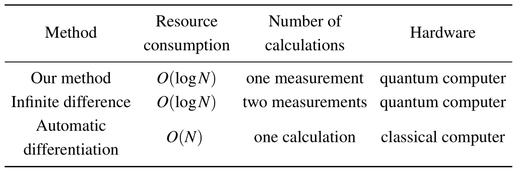
Table 1.Method comparison.
The analysis shows that the proposed method requires fewer resources and is more efficient.
4.Implementation
In this section,we construct a quantum variational circuit classifier model by using the PennyLane framework.[37]We use the MNIST handwritten digital classification dataset[38]as the training set and verification set for our model; this is widely considered as the real testbed for new machine learning paradigms.The MNIST dataset consists of hand-drawn digits from 0 to 9 in the form of gray-scale images.Each image contains 28×28 pixels, or in other words 784 features.Each feature is a integer ranging from 0 to 255 with 0 meaning the whitest and 255 the darkest color.To fit our model, a principal component analysis dimensionality reduction algorithm is used to reduce the image features from 28×28=784 to 16×16=256, so that the featuresxof one image can be encoded to a quantum state|ϕ(x)〉with 8 qubits by amplitude encoding(28=256).
The measurement of an observableMchosen from our model here is a Pauli-Zbasis measurement in one wire; such a model can be a two-category classifier.The quantum variational circuit classifier model is shown in Fig.2.
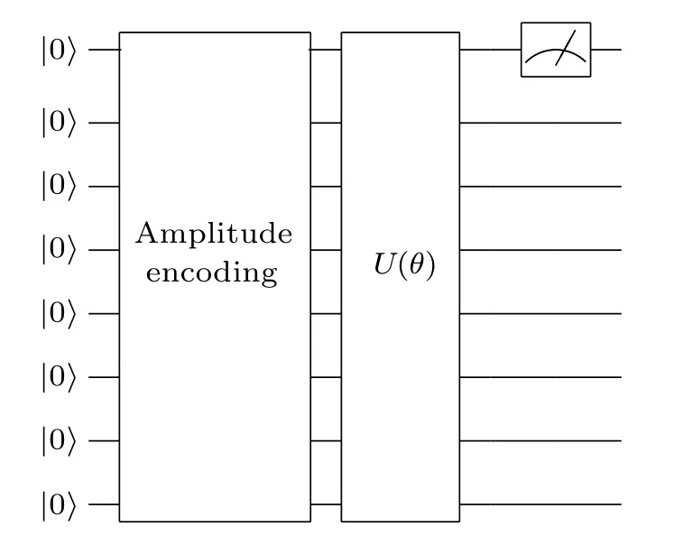
Fig.2.The quantum variational circuit classifier.The depth of U(θ) is 10,and the“amplitude encoding”can convert|0〉⊗8 to|ϕ(x)〉.
We select all images labeled 0 and 1 from the MNIST data set and choose Eq.(5) as the loss function.To train the classifier, we use the Nesterov momentum optimizer with a batch size of 10 and a learning rate of 0.05 to minimize the loss function.The average accuracy and loss as a function of the number of training steps can be seen in Fig.3.

Fig.3.The average loss and accuracy as a function of the number of training steps.
Next,we select two images labeled 0 and two images labeled 1, respectively, and they can be correctly classified by our model,as shown in Fig.4.

Fig.4.Images correctly classified by our model.
According to the method proposed in Section 3,we construct the corresponding quantum circuit to getκi, which can be seen in Fig.5,evaluate the gradient of the loss function of the four images above with respect tox,then define the value ofεrespectively, construct the adversarial examples of these four images in Fig.4 according to Eqs.(2)and(3).

Fig.5.The quantum circuit of getting κi,because the observable M chosen from our model is a Pauli-Z basis measurement in one wire,there is a control-Z gate on it.
We take the adversarial examples as the input of the model but the output of the model does not match their label,as shown in Fig.6.
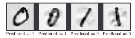
Fig.6.The adversarial examples.
Next, we construct adversarial examples for all the images labeled 0 and 1.
Although malicious attackers can attack some quantum variational circuit models by using adversarial samples, the robustness of the model can also be enhanced by using adversarial examples to train the model.Due to different images theεneeded for constructing the adversarial examples may not be at the same scale,so for measuring the difference between the legitimate and adversarial images we define fidelity between quantum states that encode the legitimate and adversarial examples:|〈ϕ(x′)|ϕ(x)〉|2.In order to give a positive role to adversarial examples, we use adversarial examples with a fidelity of 0.9 to continue training the model, and we use the Nesterov momentum optimizer with a batch size of 10 and a learning rate of 0.05 to minimize the loss function.The average accuracy and loss as a function of the number of training steps can be seen in Fig.7.

Fig.7.The average accuracy and loss as a function of the number of training steps when using adversarial examples with a fidelity of 0.9 as the training data.
Then,we compare the present model with the model that has not been trained with adversarial examples.The average accuracy as a function of the fidelity can be seen in Fig.8.
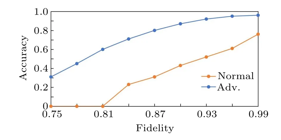
Fig.8.The average accuracy as a function of the fidelity.“Adv.” refers to the model has been trained with adversarial examples,“normal”refers to the model that has not been trained with adversarial examples.
It is obvious that the ‘Adv.’ model has higher accuracy for adversarial examples with lower fidelity,which means that the model trained with adversarial examples is more robust.
5.Conclusion
In summary, we propose a method to calculate the gradient of loss function of a quantum variational circuit with respect toxby quantum circuits,which is a key point to construct adversarial examples.Compared with the automatic differentiation method and finite difference method,our method has advantages in efficiency and resource consumption.We use the MNIST handwritten digit classification dataset to train a two-category quantum variational circuit classifier, and use the method proposed to calculate the gradient of loss function with respect toxto construct adversarial examples.These adversarial examples are predicted wrongly by the classifier.We use the adversarial examples as a new dataset to train the model,and the new model is more robust than the model without the adversarial examples training.
Acknowledgments
Project supported by the National Natural Science Foundation of China (Grant Nos.62076042 and 62102049),the Natural Science Foundation of Sichuan Province (Grant No.2022NSFSC0535), the Key Research and Development Project of Sichuan Province(Grant Nos.2021YFSY0012 and 2021YFG0332), the Key Research and Development Project of Chengdu(Grant No.2021-YF05-02424-GX),and the Innovation Team of Quantum Security Communication of Sichuan Province(Grant No.17TD0009).
猜你喜欢
早期教育(家庭教育)(2022年12期)2022-05-30
幼儿教育·父母孩子版(2020年8期)2020-03-04
环球人物(2018年19期)2018-10-17
红蜻蜓·低年级(2017年10期)2017-11-21
西江文艺(2017年15期)2017-09-10
西江文艺(2017年15期)2017-09-10
小天使·四年级语数英综合(2016年10期)2016-10-12
中国篆刻(2016年3期)2016-09-26

- Chinese Physics B的其它文章
- Interaction solutions and localized waves to the(2+1)-dimensional Hirota–Satsuma–Ito equation with variable coefficient
- Soliton propagation for a coupled Schr¨odinger equation describing Rossby waves
- Angle robust transmitted plasmonic colors with different surroundings utilizing localized surface plasmon resonance
- Rapid stabilization of stochastic quantum systems in a unified framework
- An improved ISR-WV rumor propagation model based on multichannels with time delay and pulse vaccination
- Quantum homomorphic broadcast multi-signature based on homomorphic aggregation