The limit cycle bifurcations of a cubic differential system with two invariant lines

YANG Jihua

(School of Mathematics and Computer Science,Ningxia Normal University,Guyuan Ningxia 756099)

Abstract This paper deals with the number of limit cycles of a piecewise smooth cubic integrable differential system with the switching line x=0 under perturbations of polynomials of degree n.By using the first order averaging function,we get the maximum number of limit cycles bifurcating from the period annulus surrounding the origin.

Key words Limit cycle;Averaging method;Argument Principle

The study of piecewise smooth differential systems with two invariant curves of the form

(1)

has gained increasing attention among scholars in recent years,where 0<|ε|≪1,andf±(x,y)andg±(x,y) are polynomials of degreen.For example,LI S et al.[1]studied the system (1),withμ+(x,y)=ax+1 andμ-(x,y)=bx+1.TIAN Y et al.[2]considered the case ofμ+(x,y)=ax+1 andμ-(x,y)=by+1.YANG J et al.[3]investigated the case ofμ+(x,y)=ax2+1 andμ-(x,y)=bx2+1.

In this paper,we intend to study the number of limit cycles of system (1) withμ+(x,y)=(x+a)2andμ-(x,y)=(x+b)2,whereab≠0.That is,we consider the system

(2)

where

(3)

System (2)|ε=0is a piecewise smooth integrable non-Hamiltonian system with a generalized center (0,0) and has an invariant straight line (x+a)2=0 (resp.(x+b)2=0) fora<0 (resp.b>0).Let

(4)

1 Preliminaries and main result

We first summarize some results on the first order averaging method for discontinuous differential systems.For a general introduction to the averaging method,one can consult [4-7] and references therein for details.

Lemma1 Consider the following discontinuous differential equation

(5)

with

whereF1,F2∶×D→,R1,R2∶×D×(-ε0,ε0)→,μ∶×D→are continuous functions,T-periodic in the variableθandDis an open interval of.We also suppose thatμis aC1function having 0 as a regular value.Denote byM=μ-1(0),by Σ={0}×D⊂M,by Σ0=ΣM≠∅,and its elements byz∶=(0,z)∉M.

Define the averaged functionf0∶D→as

(6)

We assume the following three conditions:

(i)F1,F2,R1,R2andμare locally Lipschitz with respect tor.

(iii) If ∂μ/∂θ≠0,then for all (θ,r)∈Mwe have that (∂μ/∂θ)(θ,r)≠0;and if ∂μ/∂θ≡0,then 〈∇rμ,F1〉2-〈∇rμ,F2〉2>0 for all (θ,z)∈[0,T]×M,where ∇rμis the gradient of the functionμrestricted to variabler.

Then for |ε|>0 sufficiently small,there exists a T-periodic solutionr(θ,ε) of system (5) such thatr(0,ε)→a(in the sense of Hausdorff distance) asε→0.

In order to verify the hypothesis (ii) of Lemma 1,we have the following remark,see for instance [4].

Remark1 Letf0∶D→be aC1function withf0(a)=0,whereDis an open interval ofanda∈D.Whenever the Jacobian ofJf0(a)≠0,there exists a neighborhoodVofasuch thatf0(r)≠0 for alldB(f0,V,0)≠0.

Lemma2[8]Considerp+1 linearly independent analytical functionsfi∶U→,i=0,1,2,…,p, whereU⊂is an interval.Suppose that there existsj∈{0,1,…,p} such thatfjhas constant sign.Then there existp+1 constantsδi,i=0,1,…,p,such thathas at leastpsimple zeros inU.

The main result of this paper is the following theorem.

Theorem1 If the first order averaging function is not identically zero,then,for anyn≥1,

2 The expression of averaged function and the lower bounds

Letx=rcosθ,y=rsinθ.Forx>0,system (2) can be written as

whereh1(r,θ)=(rcosθ+a)2.Then,we obtain that

where

Similarly,we have,forx<0,that

where

andh2(r,θ)=(rcosθ+b)2.It is known thatX±are well defined in (0,r0).Hence,system (2) is equivalent to

with

where

It is obvious thatFi(θ,r),Ri(θ,r,ε),i=1,2 andμ(θ,r)=cosθare local Lipschitz with respectr.SinceM={(r,θ)|r∈(0,r0),θ=π/2,3π/2},the function ∂μ(θ,r)/∂θ=-sinθ≠0 when (r,θ)∈M.According to the Lemma 1 and the equality (6),we need to compute the number of simple zeros of the averaged function

where

Lemma3 The following equalities hold

rAi+1,j(r)=Ii,j(r)-aAi,j(r),rBi+1,j(r)=Ji,j(r)-bBi,j(r),

(7)

(8)

(9)

ProofWe only prove the first equality in (9) by induction oni.It follows from [1] that

(10)

(8) and the first equality in (10) imply that the first equality in (9) holds fori= 1,2.Suppose that it holds fori=l.Then fori=l+ 1,noting that (10) we have that

which implies that the first equality in (9) holds fori=l+ 1.This ends the proof.

By (8),we obtain that

where

(11)

By (9),we have that

Notice that

Thus,we have proved the following lemma.

Lemma4F(r) can be expressed as

(12)

where

(13)

(ii) Sinceσi,jandτi,jare arbitrary,(11) implies thatSi,jandTi,jcan be chosen arbitrarily.

In view of Lemma 4 and Remark 2,one has the following lemma.

(ii)Ifnis an even number,then the coefficientsai,bk,cianddkin (12) are arbitrary for

In what follows,we intend to obtain the lower bounds of the number of zeros ofF(r) by Lemma 2.To this end,we will suppose thatrandF(r) are complex from now on.

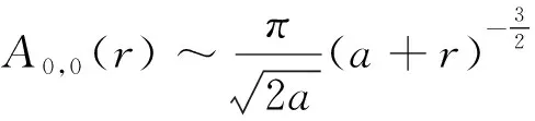
Lemma6 (i) Ifa>0,thenA0,0(r) can be analytically extended to the complex domain

D1={r∈|r≤-a}.

(ii)Ifb>0,thenB0,0(r) can be analytically extended to the complex domain

D2={r∈|r≤b}.

(14)

SoA0,0(r) satisfies the equation

(15)

Solving the above equation,we get that

(16)

(17)

(18)

wherec1andc2are non-zero real constants andi2=-1.

which implies that

Solving the above equation yields that

wherec∈is a constant.Sinceis a pure imaginary number,and we can supposec=c1i(c1∈).We claim thatc1is nonzero.Otherwise,A0,0(r) is global single-valued,andA0,0(r) will be analytic atr=-aor -ais a pole ofA0,0(r),which is a contradiction with the factwhenr→-a.

The conclusion (ii) can be shown similarly.

Lemma9 The generating functions ofF(r) are the linearly independent functions as follows:

(i) Fora≠-bandnis an odd number

(ii) Fora≠-bandnis an even number

(iii) Fora=-bandnis an odd number

(iv) Fora=-bandnis an even number

Proof(i) Suppose that

We need to prove

Ifa>0,b>0,then Φ(r) can be analytically extended to the domainD=D1∩D2.Whenr∈(-∞,-a),(17) implies that

The other cases,such asa>0 andb<0,a<0 andb>0,anda<0 andb<0 can be proved similarly.Following the same argument,we can prove (ii)-(iv).

Remark3 By Lemma 2 and Lemma 9 we obtain the lower bounds ofH(n).

3 The upper bounds

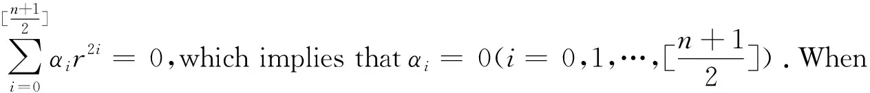
In the following we will get the upper bounds ofH(n) by using the Argument Principle.Suppose thata>0,b>0 andnis odd.Ifnis an even number,the upper bounds ofH(n) can be obtained similarly.

Fig.1.Graph of the closed curve G.