A Deep Learning Approach to Shape Optimization Problems for Flexoelectric Materials Using the Isogeometric Finite Element Method

Yu Cheng,Yajun Huang,Shuai Li,Zhongbin Zhou,Xiaohui Yuanand Yanming Xu,⋆

1College of Architecture and Civil Engineering,Xinyang Normal University,Xinyang,464000,China

2Henan Unsaturated Soil and Special Soil Engineering Technology Research Center,Xinyang Normal University,Xinyang,464000,China

3College of Intelligent Construction,Wuchang University of Technology,Wuhan,430223,China

4College of Civil Engineering and Architecture,Dalian University,Dalian,116622,China

5Henan International Joint Laboratory of Structural Mechanics and Computational Simulation,School of Architecture and Civil Engineering,Huanghuai University,Zhumadian,463000,China

ABSTRACT A new approach for flexoelectric material shape optimization is proposed in this study.In this work,a proxy model based on artificial neural network (ANN) is used to solve the parameter optimization and shape optimization problems.To improve the fitting ability of the neural network,we use the idea of pre-training to determine the structure of the neural network and combine different optimizers for training.The isogeometric analysis-finite element method (IGA-FEM) is used to discretize the flexural theoretical formulas and obtain samples, which helps ANN to build a proxy model from the model shape to the target value.The effectiveness of the proposed method is verified through two numerical examples of parameter optimization and one numerical example of shape optimization.

KEYWORDS Shape optimization;deep learning;flexoelectric structure;finite element method;isogeometric

1 Introduction

Optimization plays a vital role in the analysis of physical systems and in the science of decision making, aiming to maximize utility within resource constraints.Structural optimization problems can be broadly classified into three categories:size optimization[1–3],shape optimization[4–6],and topology optimization [7–10].Size optimization [11–13] focuses on minimizing the thickness (e.g.,cross-sectional area) of a specific structure type.Shape optimization [14–16] focuses on optimizing specific contours or shapes of designated domain boundary segments.Topology optimization[17–19]aims to minimize the material layout of the entire structure.Several approaches have been proposed to tackle optimization problems,including Newton’s method,Gauss-Newton method and some other methods [20–24].Moreover, researchers have developed metaheuristic optimization algorithms like Particle Swarm Optimization[25],Differential Evolution[26],and other similar techniques[27–30].

Machine learning has gained significant attention in recent years as an alternative to classical optimization methods[31,32].Since the 1980s,artificial neural network(ANN)[33–36]has become a prominent research topic in the field of artificial intelligence.ANN aims to simulate the information processing mechanism of neuronal networks in the human brain by constructing simplified models through various connection methods.ANN is composed of interconnected nodes,known as neurons,which represent specific output functions or activation functions.The connections between these nodes are represented by weighted values called weights, which act as the neural network’s memory.The output of the network is determined by the specific connection method,weight values,and activation functions utilized.Neural networks are often used to approximate algorithms or natural functions and to express logical strategies.

Kien et al.[37,38]proposed the Deep Lagrangian Method(DLM)as a new approach for solving size and shape optimization problems.This method cleverly combines Lagrange duality with deep learning techniques.Lagrangian duality theory provides a framework for solving the dual problems associated with primal constrained optimization problems.In the DLM,input data is utilized to train a deep neural network,with the parameters fine-tuned until the output closely aligns with the predicted values.By leveraging the interpolation capabilities of deep learning,the method effectively identifies the minimum input value.Consequently,this deep learning-based method enhances sensitivity analysis by making efficient use of a substantial amount of input data for neural network training.

Flexoelectricity was first introduced by Mashkevich and Tolpygo in 1957[39],but its significance in bulk crystal materials was found to be weak,resulting in limited attention during the early stages.However,with the advancements in nanotechnology,significant strain gradients can now be observed at small scales,leading to the emergence of flexible electronics as a new avenue for studying size-related phenomena [40,41].Unlike piezoelectric materials, where linear polarization is observed, different piezoelectric materials in flexible structures exhibit polarization that is dependent on the gradient.This makes flexoelectricity a more prevalent electromechanical coupling mechanism [42], as it can occur in any dielectric material, including those with centrally symmetric crystal structures [43–45].Chen et al.[46] used a generalized n th-order perturbation and other isogeometry stochastic finite element method to quantitatively analyze the uncertainty of the mechanical properties of piezoelectric materials.

In the realm of flexoelectric effect analysis,numerous scholars have made remarkable contributions.El Dhaba et al.[47] and Awad et al.[48] examined the flexoelectric effects of materials with anisotropy and isotropy, correspondingly.Ghasemi et al.[49] introduced an isogeometric formula to calculate the flexoelectric effect based on the strain gradient expression of flexoelectricity, and presented 2D cantilever and 3D truncated pyramid models.Qu et al.[50] conducted a study on the buckling of piezoelectric semiconductor Reissner Mindlin plates.They determined the buckling load and mode,and also examined the wave particle resistance effect of flexible semiconductor materials[51].Nguyen et al.[52] developed an isogeometric numerical model for the Maxwell-Wagner polarization effect in bilayer structures consisting of piezoelectric or flexoelectric materials.Liu et al.[53]constructed a real spatial phase field model using isogeometric analysis (IGA) to investigate the flexoelectric effect of ferroelectric materials at the nanoscale.Yin et al.[54]derived a curvature-based Euler-Bernoulli and Timoshenko beam model for flexoelectricity based on the coupled stress and flexoelectricity theory.They analyzed the impacts of flexoelectric effects,microstructure effects,and boundary conditions on the mechanical behavior of nanobeams using IGA.Gupta et al.[55]explored the effective piezoelectric and dielectric properties of boron nitride(BN)reinforced nanocomposites(BNRC), along with the surface flexoelectric effect.Their findings indicated that size-dependent flexoelectric and surface effects should be taken into account for accurate modeling of active nanostructures.

IGA represents substantial progress in computational mechanics[56],functioning as an expansion of the finite element technique.One of the key advantages of isogeometric analysis (IGA) is its ability to discretize partial differential equations using non-uniform rational B-spline basis functions.This feature allows engineers to directly perform numerical analysis from computer-aided design(CAD)models[57–61],ensuring both geometric accuracy[62–65]and eliminating the need for mesh generation.It is worth mentioning the contributions made by Jahanbin and Rahman[66]in developing engineering applications for uncertainty quantification through Stochastic Isogeometric Analysis(SIGA)in high-dimensional linear elasticity.Furthermore,Liu et al.[67]proposed a novel technique based on reduced basis vectors in SIGA for solving practical engineering problems.Chen et al.[68]utilized the radial integration technique for solving 2-D transient heat conduction problems via isogeometric boundary element analysis.Due to IGA’s ability to meet the continuity requirements of fourth-order partial differential equations (PDEs), it becomes possible to consider the flexible electrical properties by ensuring the necessaryC1continuity [69].As a result, this article selects isogeometric analysis-finite element method(IGA-FEM)as the method for obtaining the mechanical properties of flexible electrical structures.

Based on the aforementioned inspiration,we propose a method that combines ANN and IGAFEM for solving shape optimization problems.In this method, the bending theoretical formulas are discretized using IGA-FEM to generate samples.These samples are then used to train the artificial neural network,which establishes a proxy model linking the model shape to the target value.Subsequently,this proxy model is utilized to solve shape optimization problems.

The content structure of this paper is set as follows: In the second section, the steps and improvements of ANN for optimization problems are introduced.In the third section,the theoretical formulas of flexographic problems and how to obtain initial samples by IGA-FEM method are expounded.Finally, in the fourth section, the effectiveness and accuracy of the method are verified by numerical examples.

2 Artificial Neural Network Methods for Optimization Problems

In order to make it easier for readers to understand, we first give a brief introduction to the composition and working principle of ANN.Please see[70–72]for detailed information.

2.1 Artificial Neural Network

ANN typically consist of three layers: input, hidden, and output.Among them, the input layer receives data,while the output layer produces the final result.Multiple hidden layers can exist.Each layer contains multiple neurons, with the number depending on specific requirements.The number of hidden layers in ANN can be customized, often involving multiple layers.These layers are fully connected,meaning that there are connections between adjacent layers,but no connections within the same layer.

Neural networks utilize two main processes,known as forward propagation and back propagation,to achieve self-learning.Forward propagation involves inputting samples into the neural network,which then passes through hidden layers until the output layer generates the desired output.The quality of the model’s fit is evaluated by assessing the loss function.Typically,the mean square error between the output layer results and sample labels is commonly utilized as the loss function for ANN,Fig.1 illustrates an ANN network structure and neuronal node calculation process.

Figure 1:Neural network structure and neuron parameters

The input and output vectors are denoted asx= {X1,X2,...,Xn0} andp=(X1,X2,...,Xn0),respectively.Each node establishes connections with the subsequent layer via weight vectorsωand bias termsb.The activation Functionfkis used to calculate the output value of neurons located in thek-th hidden layer,as shown as

where i=1,2,...,nk,1 ≤k ≤K,K is the total number of the hidden layers.At the first layer,we have

where i=1,2,...,nk.At the last layer,we have

where i=1,2,...,nK.The weights and biases are represented asωijandbi,respectively.The node’s position within the layer is denoted by j,andnk-1represents the total number of neurons in the(k-1)-th layer.Therefore,the output can be expressed as

In this study,we employed ANN to address the optimization problem.The methodology involved constructing a surrogate model of the optimization problem by training an artificial neural network,in order to find the optimal solution to the optimization problem.Notably,the ANN method is wellsuited to address nonlinear optimization problems,thus enhancing its capability in handling complex systems.For instance,

Then,the mapping model ofx={x1,x2,...,xn}to0(x)is established through the neural network,so the optimization problem(FL)can be written as

Using the mapping capabilities of neural networks,the initial sample can be expanded to

2.2 Dual Optimization Neural Network(DONN)

The accuracy of models in artificial neural networks during training and prediction is influenced by the neural network structure, including hidden layers and neurons.However, the optimal neural network structures vary for different problems.To address this,we propose a data-driven approach,referred to as Algorithm 1.This approach efficiently discovers a neural network structure that is better suited to the specific model,reducing the required time.The implementation concept of the algorithm is provided in the appendix in Fig.A1.

The DONN method first determines the optimal combination of a set of neural network layers and neurons through Algorithm 1 to establish a neural network structure,and then inputs the training data setsinto the neural network for training,and obtainstomapping relationship.After that,predict enoughto get,find the minimum value inand its correspondingcombination.

The sigmoid function serves as the activation function for neuron nodes.Let us assume that the predicted value of thej-th unit in the output layer is represented as.In order to quantify the loss,the Mean Square Error(MSE)is chosen as the loss function and can be formulated as

Thus,as the value of the loss function approaches zero,the neural network’s predicted result and the actual result exhibit a smaller error.The role of a neural network optimizer is to continuously minimize the loss function through training on the data set.Different optimizers possess varying capabilities in reducing the loss function’s value.Furthermore, the choice of optimizer depends on the specific problem at hand,as different problems may require different optimizers.An appropriate optimizer not only enhances model accuracy but also minimizes the required training iterations and mitigates the risk of overfitting the neural network.In practice, it is possible to employ multiple optimizers for combined training within a neural network.Selecting the appropriate number of iterations further enhances training efficiency.

We divide the process of stochastic analysis with DONN into three stages:

(1) Preparation stage: Obtain a batch of training data sets through Latin-Hypercube sampling,leave samples that meet the constraints, obtain the initial data setX,Y.After normalization, the training setis obtained.The normalization process is expressed as follows:

A small part of the normalized dataset is selected,and an artificial neural network is established through Algorithm 1.

(2) Model training and validation phase: the dataset is divided into training dataset and testing dataset.The former is utilized to construct the approximate function f that captures the relationship between the input and output.The latter is employed to assess the model’s generalization capability.The training process of the machine learning model involves searching for optimal parameters that minimize the loss function,while the testing process is conducted to validate the accuracy of the fitted function.Furthermore,it is necessary to post-process the predicted value to ensure its alignment with the inputY.The post-processing for this purpose is provided as

wherePostXξrepresents X after de-normalization,Xmin,andXmaxrepresent the minimum and maximum values in X,respectively,andYminandYmaxrespectively represent the minimum and maximum values of Y.andrepresent arbitrary elements inand,respectively.

(3) Application stage: The correctness of the mapping relationshipis established and verified through the previous stage.Once the new normalized dataNXξis input and passed to the trained model, the response of the corresponding normalized dataNYξwill be obtained.For optimization problems, we generally want to obtain a set of parameters under the condition that the constraints are satisfied, so that the function value corresponding to this set of parameters is the maximum or minimum.

For the input variableX, if the conditions are met, selecting a relatively large value range can not only ensure that the optimal solutiong0is within this range,but also improve the accuracy of the training model, but it will also bring relatively large sample data set, increasing the computational cost.At the same time, the collected samples may not meet the constraints of the specific problem.Therefore, we perform a screening on the initial samplesX,Yobtained by using Latin hypercube sampling,in which the samples that meet the constraints are added to the training data.In this way,the scale of the dataset can be greatly reduced,and the interference of model training by irrelevant data can be reduced,thereby improving the speed and accuracy of model training.On the premise that the correctness of the model has been verified before,in order to find a more accurate optimal solution,it is a good choice to use a test set with a relatively large amount of data to find the optimal solution.The calculation speed is very fast,and there is no need to worry about increasing the computational cost.Fig.2 shows the specific operation flow chart of the DONN method.

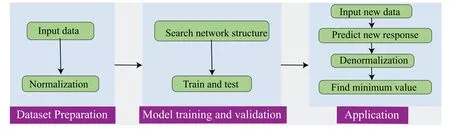
Figure 2:DONN flow charts for stochastic analysis

In the upcoming section, we will present an overview of the flexoelectric problem theory and provide guidance on obtaining the initial sample.

3 Initial Sample Acquisition for Flexoelectric Problems

In this section,we provide a comprehensive introduction to the theory of the flexoelectric problem and outline the process of obtaining initial samples using the IGA-FEM method.

3.1 Theory and Formulations of Flexoelectricity

The enthalpy densityHof dielectric materials subject to flexoelectric effects depends on both the strain gradient and the electric field gradient.The enthalpy density equation may be expressed as[73]

Using the symbolϕ,one may represent the scalar electric potential.The strain tensor is denoted by the symbolSij,whereas the fourth-order elasticity tensor is denoted by the symbolCijkl.eijkrepresents the third-order piezoelectric tensor.The signEi(i.e.,Ei=ϕ,i) stands for the electric field, which is defined as the gradient of the scalar electric potentialϕ.The symbol for the second-order dielectric tensor isκij.The symbol for the fourth-order converse flexoelectric tensor isdijkl,whereas the symbol for the fourth-order direct flexoelectric tensor is.

Consider the terms in Eq.(14)’s bracketed sections,which cover the direct and opposite flexoelectric effects.We reach the following results by integrating these terms across the physical domainΩ,using integration by parts,and using the Gauss divergence theorem to the first term.

where the single material tensorμijklis defined asμijkl=diljk-.Therefore,we can rewrite Eq.(14)as

For purely piezoelectric dielectrics,we have

The normal electromechanical stresses(),higher-order electromechanical stresses,and physical electromechanical stresses(Tij/Di)are defined by the following equations in the presence of flexoelectricity.

After substituting Eqs.(18)and(19)into Eq.(20),we obtain

The electrical enthalpy of a flexoelectric dielectric is given by

The work done by external forces, such as mechanical tractioniand surface charge density,can be expressed as

where the signuistands for displacement.represents mechanical traction,whilerepresents surface charge density.The symbolsΓtandΓDrepresent the mechanical and electric displacement boundaries,respectively.

The kinetic energy of a system is defined as

To fulfill Eq.(31) for all possible values ofu, the time integration integrand must disappear,resulting in

The inertia element is ignored in the case of a static situation,resulting in the following:

We may derive the weak version of the governing equation for flexoelectricity by putting Eqs.(18)–(22)into Eq.(33),as illustrated as

3.2 IGA-FEM Used to Discretize the Fourth-Order Partial Differential Equation of Flexoelectricity

In this section,we use B-spline basis functions to discretize the controlling Eq.(14).The B-spline basis function H is defined recursively by the Cox-de-Boor formula[74–77],and its expression is

whenp=1,2,3,...,we have

Fig.3 shows a particular multidimensional B-spline form function that is distinguished by knot vectorsΞ= [0 0 0 0 0.5 1 1 1 1].The orderspandqof the shape functions are three.The image shows that a variety of function types for the B-spline basis functions may be obtained by defining the knot vectorsΞand the ordersp,q.This meets the criteria for continuity needed to solve the governing equations for flexoelectricity.Eq.(34)’s linear algebraic discrete system equation may be stated as

Figure 3:The schematic diagram in illustrates the B-spline shape functions with a specific configuration of knot vectors

In Eqs.(38)–(43),the subscripterepresents theethfinite element inΩe,Γte,andΓDe,whereΩ=∪eΩe.The matrices Bu,Bϕ,and Huare provided as

In Eqs.(44)–(46),the subscriptncprepresents the the number of basis functions.The matricesC,κ,e,andμcan be expressed in matrix form as

where the Poisson’s ratio is denoted by the symbolνand the Young’s modulus by the sign.Following that, various numerical examples are provided to demonstrate the efficacy and precision of the suggested approach.

4 Numerical Examples

In this section,we use three models to analyze the optimization problem,the first two models to analyze the parameter optimization problem, and the last model to analyze the shape optimization problem using the f lexoelectric effect as an example.

4.1 Example of Structural Parameter Optimization

First example,we examine a truss structure consisting of bars with Young’s modulus E and densityρ.The truss incorporates two connected bars,which converge at an angle ofα(as depicted in Fig.4),with the length of the first bar represented as l.A force F, greater than zero, is exerted on the truss.The problem’s objective concerns the determination of the cross-sectional areaAito achieve optimized weight.In addition, the constraint conditions for maximum stress and displacement at the tip are defined asδ.

Figure 4:A two-bar truss constrained by stress and displacement at the top

The weight of the truss is given by

In addition,the following constraints were applied to the stress:

and the displacement

We use the Latin hypercube sampling method for initial sampling,and remove the sample points that do not meet the constraints to obtain S1,which is substituted into the neural network as a training set for model training.The number of hidden layers of the neural network and the number of nodes per layer are determined by Algorithm 1.Fig.5 shows the neural network structure determined by Algorithm 1.During training,we set up a two-layer optimizer,first using the Adam optimizer for fast fitting of the pre-model,and then using the gradient descent optimizer for fine-tuning the model.The gradient descent optimizer has a learning rate of 10-4, which is used to ensure the accuracy of the model predictions.

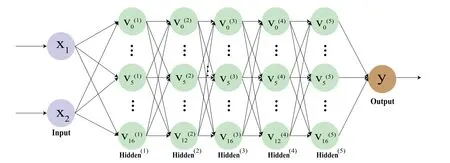
Figure 5:The first neural network structure built

In the neural network, the size of the data set directly affects the time spent in model training and the training effect.If the data set is too large,more iterations are required in the neural network training stage,and the time consumption increases significantly.At the same time,if the dataset is too small,the neural network will not be able to learn all the features,resulting in poor prediction effect after model training.Therefore,choosing a dataset of suitable size can effectively solve the above two problems.Fig.6a shows the relationship between the loss function value of different optimizers and the number of iterations,and Fig.6b shows the error curve under different sampling intervals,that is,different data sets of different sizes.

Figure 6:Decline curve of loss function and error analysis of data sets of different sizes

As can be seen from Fig.6b,whenΔX=0.001 or less,the relative error reaches the minimum.In order to shorten the training time,we chooseΔ=0.001 for sampling.After screening,2450 samples are used as the training set.SelectΔ=0.0001 for sampling.After screening,24,500 samples are used as the test set,which can not only verify the effect of training,but also verify the generalization performance of the model and help us find the optimal solution.Figs.7a and 7b show the relationship between the relative error(RE)between the predicted value and the true value and the number of iterations is given,respectively.

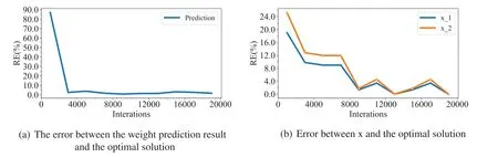
Figure 7:Error of DONN optimization results

After observing the decreasing law of the loss function and the relationship between the relative error and the number of iterations under different data and sizes,we make Adam optimizer perform 20,000 iterations,and GD optimizer perform 20,000 iterations.We restrict the range ofxito 0.01 ≤x1,x2≤3, because the optimal result is within this range.If you choose a large range ofxi(e.g.,0.01 ≤xi≤10).It will bring a lot of unnecessary calculations.

Using 1957 constrained samples as the training set,the solutions for DONN are given in Table 1,which are in good agreement with the exact solutions.

Table 1: Comparison of DONN results and analytical solutions

4.2 Weight Minimization of a Cantilever

Second example,we shift our focus to the cantilever beam illustrated in Fig.8.The beam possesses a thin-walled cross-section depicted in Fig.8b,with a thickness labeled as t.Each segment of the crosssection has a side length denoted asxi,where i=1,2.The objective is to determine the values ofxithat optimize the weight of the cantilever beam while ensuring that the tip displacement,δ,remains below a specified threshold denoted asδ0[78].

Figure 8:Cantilever structure(a)and hollow square section(b)

In this case,we make an assumption that the thickness of the segment is significantly smaller in comparison to the side length, denoted ast≪xi.As a result, the second moment of inertia can be calculated as

Then,the weight of the beam can be calculated using the following equation:

The calculation of tip displacement can be expressed as[78]

The optimization problem of nested formulas can be expressed as follows:

In Table 2,the results of the DLM methods can be found.

Table 2: Comparison of DONN results and analytical solutions

Table 3: Parameter setting table of truncated pyramid

Table 4: Table of characteristic parameters of conical materials

Similar to the previous example, we set the range forxiagain, 0.1 ≤x1,x2 ≤5, to ensure the global minimum value; the neural network structure determined by Algorithm 1 is shown in Fig.9.Fig.10 shows the change curves of loss functions for different optimizers and the relative error curves of optimization results for data sets of different sizes.After observing the decreasing law of the loss function and the relationship between the relative error and the number of iterations under different data and sizes, we made the Adam optimizer perform 20,000 iterations and the GD optimizer for 20,000 iterations.We chooseΔ= 0.001 for sampling, and after filtering, 2450 samples are used as training set S2.SelectΔ=0.0001 for sampling,after screening,take 24,500 samples as the test set,S2,input S2 as the training set into the neural network for model training,and find the smallest predicted value from the test set A set of{x1,x2,y}.The DLM solution is given in Table 2,which agrees well with the exact solution.Figs.11a and 11b show the relative error(RE)between the predicted and true values as a function of the number of iterations,respectively.

Figure 9:The second neural network structure built

Figure 10:Decline curve of loss function and error analysis of data sets of different sizes

Figure 11:The relationship between the error of the predicted result and the true value and the number of training times of the neural network

4.3 Shape Optimization of Flexoelectric Materials

The shape of flexoelectric materials that is most frequently researched is the truncated pyramid.In Fig.12, the truncated pyramid model is displayed.While the bottom edge is immovable, the top edge is subject to evenly distributed forces ofFmagnitude.Tables 3 and 4 provide the dimensions of the model and the characteristics of theBaTiO3material used,respectively.Here,we specifically state that the top edge’s electric potential is zero.Here,we process the electric potential at the bottom edge using the penalty function technique,leading to an equipotential border condition.We get the electric potential and strain distributions shown in Fig.13 for this benchmark scenario.The distributions of the electric potential and strain are largely identical to those seen in[79].

Figure 12:The size of the truncated cone model structure and the uniformly distributed force on the upper edge

Figure 13:The distribution of total potential(a)and the distribution of strain in the x2 direction(b)

Firstly,we add control points to the truncated pyramid shape in Fig.14.Then,we use the control points on the two waists of the trapezoid as input parameters for ANN and change them within a range of 20 percent,the maximum potential corresponding to the initial truncated pyramid is 0.374193.Using ANN,we find a shape with a larger potential than before.

Figure 14:The truncated pyramid shape control point and its movement direction,with points within the dashed line as random variables,vary within a 20 percent range

In terms of sample calculation, we select three control points on each waist, so that their xdirection coordinates fluctuate within a 20 percent range.5000 sets of samples were calculated using IGA-FEM, and an ANN network was trained 50,000 times to obtain a mapping model of the maximum potential corresponding to the shape from the control point coordinates.The loss values of ANN are given in Fig.15a,and the prediction error is shown in Fig.15b.

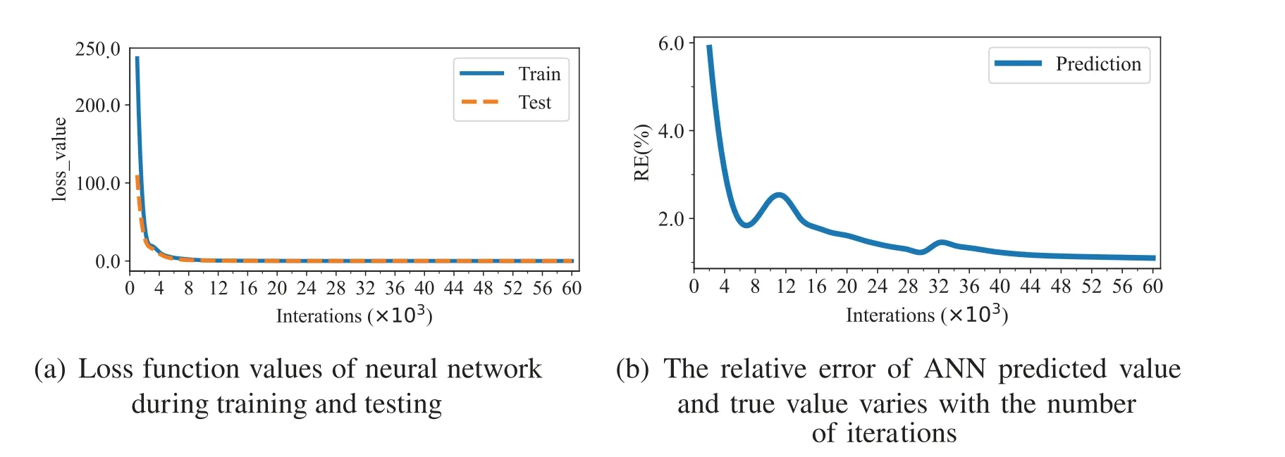
Figure 15:Loss function decline curve(a)and relative error curve(b)between predicted value and true value during ANN training

It can be seen from the prediction error chart of loss value that the prediction error of neural network reaches a very low degree.Therefore, it can be used for the shape optimization of this problem.The shape change in the optimization process is shown in Fig.16, The corresponding potential and strain distributions are given in Figs.17 and 18,respectively.In addition,Fig.19 shows the optimization effect curve under different training times.

With the increase of the number of iterations, the prediction accuracy and optimization effect of the neural network gradually increased,and became stable after the number of iterations reached 32,000.

Figure 16:The shape obtained by optimization under different iterations

Figure 17:The potential distribution corresponding to the shape is optimized under different iterations

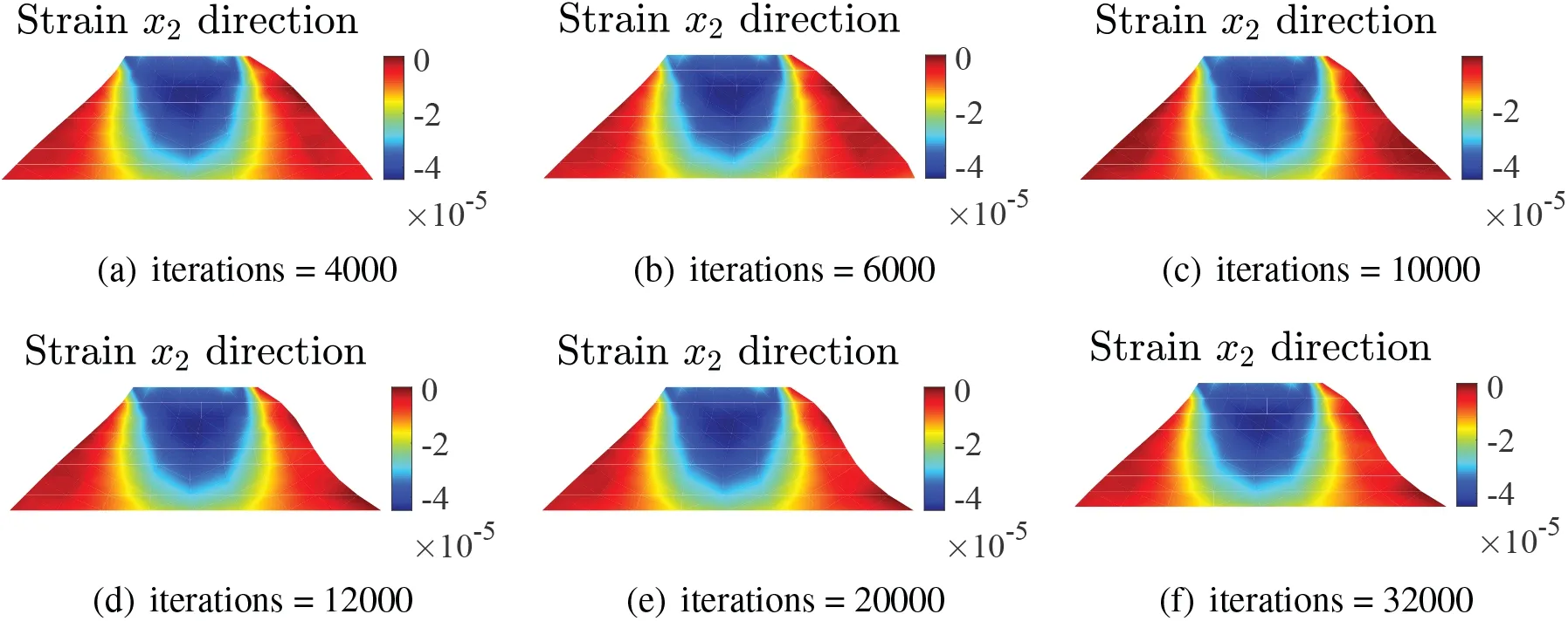
Figure 18: The displacement distribution corresponding to the shape is optimized under different iterations

Figure 19: The maximum potential value corresponding to the optimized shape under different iterations(a)and the percentage increase of the optimized maximum potential value compared with the original model(b)

5 Conclusion

In this paper,ANN is used to optimize the structural parameters and shapes,and some techniques to improve the fitting effect are proposed.ANN only needs the samples of the corresponding problem for optimization,and then a proxy model could be built to deal with the optimization problem.Since the reliability of the optimization in this method depends on the accuracy of ANN, the idea of pretraining is used to find a suitable network structure,and the method of combining multiple optimizers is used to improve the prediction accuracy of ANN.To ensure the accuracy of samples,IGA-FEM is used to obtain high-precision samples,and the mapping model from shape control points to maximum potentials is established to solve the shape optimization problem.In the future,we will introduce deeper neural networks and meta-heuristic optimization algorithms,and study the extension of this method to shape optimization problems of more complex models.

Acknowledgement:The authors wish to express sincere appreciation to the reviewers for their valuable comments,which significantly improved this paper.

Funding Statement:The research in this article has been supported by a Major Research Project in Higher Education Institutions in Henan Province,with Project Number 23A560015.

Author Contributions:The authors confirm contribution to the paper as follows: study conception and design:Yu Cheng,Yajun Huang,Xiaohui Yuan;data collection:Yu Cheng,Shuai Li,Zhongbin Zhou;analysis and interpretation of results:Yu Cheng,Yajun Huang,Yanming Xu;draft manuscript preparation:Yu Cheng,Xiaohui Yuan,Yanming Xu.All authors reviewed the results and approved the final version of the manuscript.

Availability of Data and Materials:Data is available on request.

Conflicts of Interest:The authors declare that they have no conflicts of interest to report regarding the present study.

Appendix A

Figure A1:Algorithm 1:Neural network structure random search algorithm