A Mean-Field Game for a Forward-Backward Stochastic System With Partial Observation and Common Noise

Pengyan Huang , Guangchen Wang ,,, Shujun Wang , and Hua Xiao

Abstract—This paper considers a linear-quadratic (LQ) meanfield game governed by a forward-backward stochastic system with partial observation and common noise, where a coupling structure enters state equations, cost functionals and observation equations.Firstly, to reduce the complexity of solving the meanfield game, a limiting control problem is introduced.By virtue of the decomposition approach, an admissible control set is proposed.Applying a filter technique and dimensional-expansion technique, a decentralized control strategy and a consistency condition system are derived, and the related solvability is also addressed.Secondly, we discuss an approximate Nash equilibrium property of the decentralized control strategy.Finally, we work out a financial problem with some numerical simulations.

I.INTRODUCTION

THE stochastic differential game problem within largepopulation system has attracted increasing attentions from various areas.A large-population system is distinguished with numerous agents, where the states or the cost functionals are coupled via a coupling structure.In view of the highly complicated coupling term, it is not feasible or effective to study the exact Nash equilibrium relying on all agents’ exact states.Alternatively, an available and effective idea is to design an approximate Nash equilibrium only based on each individual’s information.The mean-field method independently proposed by [1] and [2] provides an effective technique to solve the large-population game problem.With the mean-field method,a complex mean-field game problem can be converted into a series of classical control problems; as a result, the curse of dimensionality is overcome and computational complexity is reduced.Reference [2] studied a mean-field game, where the dynamic systems are asymmetric, and the analysis for theϵ-Nash equilibrium was given.Reference [3] established some results showing the unique solvability of stochastic mean-field games.Some recent works can be found in: [4], [5] for meanfield games with the Stackelberg structure, [6]-[8] for game models with the linear-quadratic (LQ) framework, [9]-[11]for game models with jumps, [12]-[14] for game models with state or control constraints, [15], [16] for game problems with social optimality, [17], [18] for backward stochastic meanfield games, [19] for Nash equilibriums of game problems,and [20]-[24] for stochastic mean-field control problems.

We point out that in the mean-field game, there are numerous agents with complicated interactions, and the state-average is approximated by a frozen term; thus, the optimal strategy can be computed off-line.However, in the mean-field control problem, the mathematical expectation of state is a part of the state, which is influenced by the control process.As a result, the strategies derived from a mean-field game and mean-field control are calledϵ-Nash equilibrium and optimal control, respectively.

Note that the mentioned works above focus on the meanfield game problem governed by a stochastic differential equation (SDE) or backward SDE (BSDE).However, we often encounter such a scenario in reality.For example, the wealth level and education investment level satisfy an SDE and a BSDE (see Section V), respectively.It is well known that forward-backward SDE (FBSDE) is a well-defined dynamic system, which provides a tool to characterize and analyse the problem above.A coupled (fully or partially coupled) FBSDE involves the feature of both SDE and BSDE, and it is a combination of them in structure, which may degenerate to either one if the other vanishes.Furthermore, FBSDE is applied to illustrate many behaviors of economics, finance and other fields, such as large scale investors, recursive utility, etc.

In some existing mean-field game literature, the authors assume that all agents can access the full information.However, in reality it is unrealistic for agents to do so.Due to the dynamic system, the agents need to make decisions based on real-time information.For example, in an integrated energy system [25] affected by weather, temperature and humidity, it is difficult to guarantee the accuracy of measured data.Thus,the study of the control and game problem with incomplete information has important practical value; one can refer to[26]-[30] for more information.

Inspired by the content above, we study a mean-field game governed by FBSDE with partial observation and common noise, which plays a vital role in both theoretical research and practical application.Although there are some existing works on a mean-field game with an incomplete information scheme,this work presents many advancements.In order to avoid confusion, we list the differences and contributions of this work item by item.

1) The large-population system is more general in the paper.In this work, the dynamic system is more general than that of[31], [32], where the diffusion term Zi(·) (see (1) below)enters the drift term of BSDE.It is well known that the solution of BSDE is a pair, which has two parts, the backward state and the diffusion term.The analysis and processing of the diffusion term is challenging, and thus it is usually absent from the drift term in many research works.As a consequence, the resulting Hamiltonian system involves fully coupled conditional mean-field FBSDEs, and it is extremely challenging to solve.In order to overcome this difficulty, employing convex analysis theory, we prove the unique solvability of Problem II and the optimality system.Moreover, [33] studied a mean-field game driven by BSDE with partial information,and derived anϵ-Nash equilibrium via the stochastic maximum principle and optimal filtering.

2) Compared with [33], the state of this paper is governed by an FBSDE with partial observation instead of a BSDE with partial information.The BSDE studied in [33] is usually used to describe some financial problems with prescribed terminal conditions, which can not characterize the recursive utility optimization problems, principal-agent problems in continuous time, etc.FBSDE provides an effective tool to investigate the above problems.Employing the optimal filter technique,decomposition technique and dimensional-expansion technique, we obtain a feedback form of the decentralized control strategy relying on the optimal filter of the forward state instead of backward state given in [33].

3) Different from [31], employing a dimensional-expansion technique and introducing two ordinary differential equations(ODEs), we obtain the solvability of the consistency condition.Since the initial and terminal conditions of consistency condition (20)-(25), (27), (28) and (34) below are mixed, their solvability is extremely difficult to derive.By virtue of the dimensional-expansion technique and two ODEs, the solvability of the consistency condition is derived.However, the solvability of the consistency condition in [31] is discussed by a contraction mapping technique with a strong assumption, and it holds in some special cases.Thus, our results obtained are more universal.

4) Unlike [27], by virtue of Riccati equation approach, we obtain a feedback form of the decentralized control strategy.Introducing eight ODEs, we decouple the complicated Hamiltonian system, and propose a feedback form of the decentralized control strategy.However, [27] gave an open-loop form of the optimal control via the stochastic maximum principle.

5) Last but not least, this work significantly improves the description and resolution of the mean-field game with partial observation.In addition, this work compensates for the deficiencies and flaws, and the results obtained are more elaborate and rigorous than some existing works.See [32] for more results regarding a mean-field game with partial observation.

The rest of this paper is structured as follows.We formulate a mean-field game problem in Section II.We investigate a limiting control problem associated with an individual agent,providing a decentralized control strategy via the consistency condition and optimal filter in Section III.Section IV is dedicated to theϵ-Nash equilibrium property of a decentralized control strategy.We give a financial example and provide some remarks in Sections V and VI, respectively.

II.PROBLEM FORMULATION AND PRELIMINARY

game Problem I, whose main process is addressed as follows.Employing the mean-field method, we convert the game Problem I into a limiting control Problem II.Decoupling the optimality system, we propose a decentralized control strategy via the consistency condition, whose approximate Nash equilibrium property is also verified with FBSDE theory.

III.A LIMITING CONTROL PROBLEM

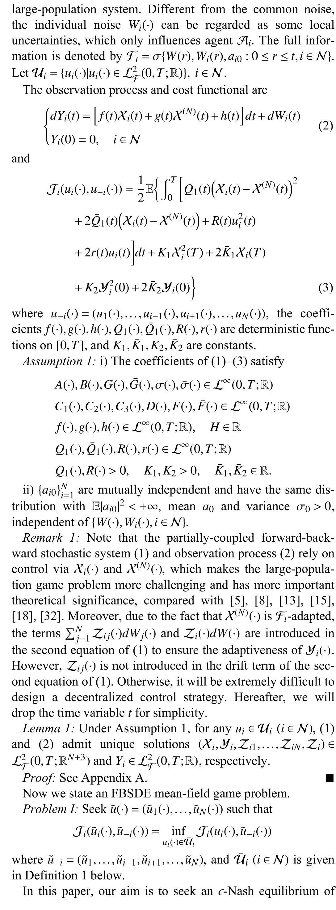
This section aims to investigate a limiting control problem associated with Problem I.Due to the common noiseW, we employ an FtW-adapted and L2- bounded stochastic processx0to approximate X(N)asN→+∞.

Introduce a limiting state equation

a limiting observation process and a limiting cost functional

and

It is easy to determine that (6)-(9) are uniquely solvable.Introduce

Itô’s formula and (6)-(10) imply that (xi,yi,zii,zi) andY¯iare the unique solutions of (4) and (5).

Let

wherePis given by Bernoulli equation

which admits a unique solution.

To investigate Problem II, we present the following lemma first, which tells us that Problem II is uniquely solvable with Assumption 1.

Lemma 2: Let Assumption 1 hold.Then, Problem II has a unique decentralized control strategy.

Proof: See Appendix B.■

Employing the classical variational method, we get

Lemma 3: Under Assumption 1, we have

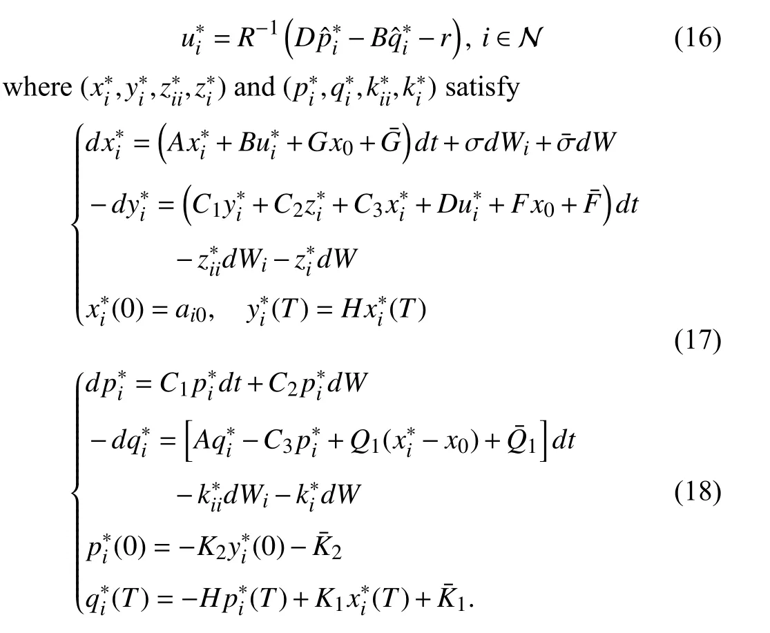
Equations (16)-(18) are called the optimality system of Problem II.By Lemma 2, Problem II is uniquely solvable,which signifies the unique solvability of (16)-(18).In what follows, we aim to decouple (17) and (18).

Assumption 2: 1 +π1(t)π4(t)≠0, where π1,π4are given by(24) and (27) below, respectively.

Theorem 1: Under Assumption 1, (17) and (18) admit unique solutions with (16).Moreover, we have the relations as follows:

i)

where

ii)

where

iii)

where

iv) With Assumption 2, we have

Proof: See Appendix C.

Remark 2: Note that (20)-(24) are independent of Ex0, in the light of Proposition 4.2 in [36], Riccati equation (20) is uniquely solvable.Then (21), (23) and (24) are uniquely solvable.Moreover, Bernoulli equation (27) results in a unique solution.However, (22), (25) and (28) depend on Ex0, whose solvability will be given in Lemma 4 below.

Theorem 2: Under Assumptions 1 and 2, we get

where

Proof: Inserting the first equality of (19), (26) and (29) into(16), we obtain feedback form (30) with (32).Moreover, it follows from (5) and (14), (31) holds.■

Remark 3: We point out that Problem II is distinguished from [27] mainly in two aspects.i) The admissible control set contains the common noiseW.Due to the presence ofW, we constructtheadmissible control setU¯idependingonWin Definition 1.Otherwise, onceWisabsentfrom U¯i,Lemma1 will not hold.Without such equivalence, it turns out to be really difficult and challenging to study Problem II.ii) Introducing eight ODEs shown in Theorem 1, we get the decentralized control strategy in a feedback form, instead of an openloop form given by [27].

In what follows, we analyse the limiting processx0and(22), (25) and (28).Introduce the decentralized control strategy:

Inserting (33) into the first equation of (1), we have

which implies that

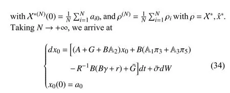
where we approximatexˆ*(N)byx0, and it will be proven in Lemma 6 below.Equations (20)-(25), (27) and (28) together with (34) are called the consistency condition.

Taking E [·] on both sides of (34), it yields

Assumption 3: We assume thatU(·) is invertible, whereU(·)is given in Appendix D.

Lemma 4: Under Assumptions 1-3, (22), (25), (28) and (35)are solvable.

Proof: See Appendix D.

According to the analysis above, limiting equation (34) is solvable, and its solutionx0is FtW-adapted and L2-bounded.

IV.ϵ-NASH EQUILIBRIUM OF PROBLEM I

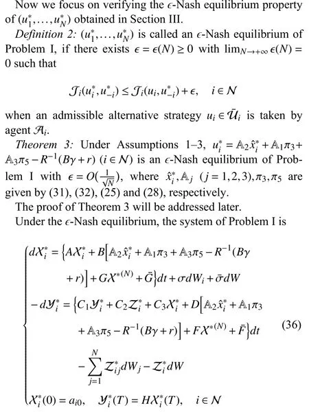
and the corresponding system of Problem II is

where

Now we summarize the process of seeking anϵ-Nash equilibrium of Problem I, which also shows the process of searching for the optimal (decentralized) control strategy (see Fig.1 below for convenience): i) Firstly, employing mean-field method, we obtain an auxiliary Problem II.ii) Secondly, by virtue of optimal filter technique, decomposition technique and dimensional-expansion technique, we obtain an optimal(decentralized) control strategy.iii) Finally, applying the FBSDE theory, we verify the decentralized control strategy obtained is anϵ-Nash equilibrium of Problem I.Moreover, the process of verifying asymptotic optimality can be illustrated by Fig.2 below.

V.A FINANCIAL EXAMPLE

In this section, we discuss a financial problem, which facilitates the study of mean-field game Problem I.

Suppose that there areNcounties in province P, in general

Fig.1.The research route.

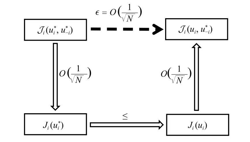
Fig.2.The process of verifying asymptotic optimality.

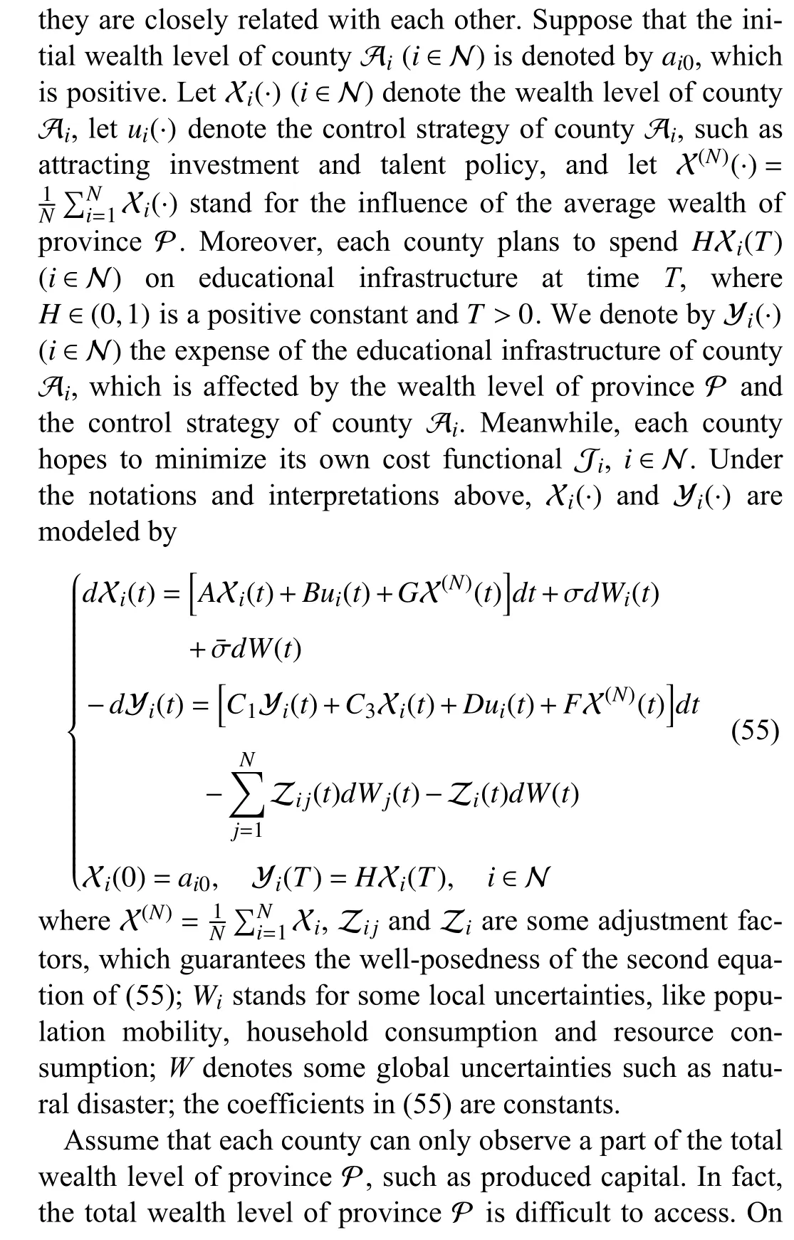
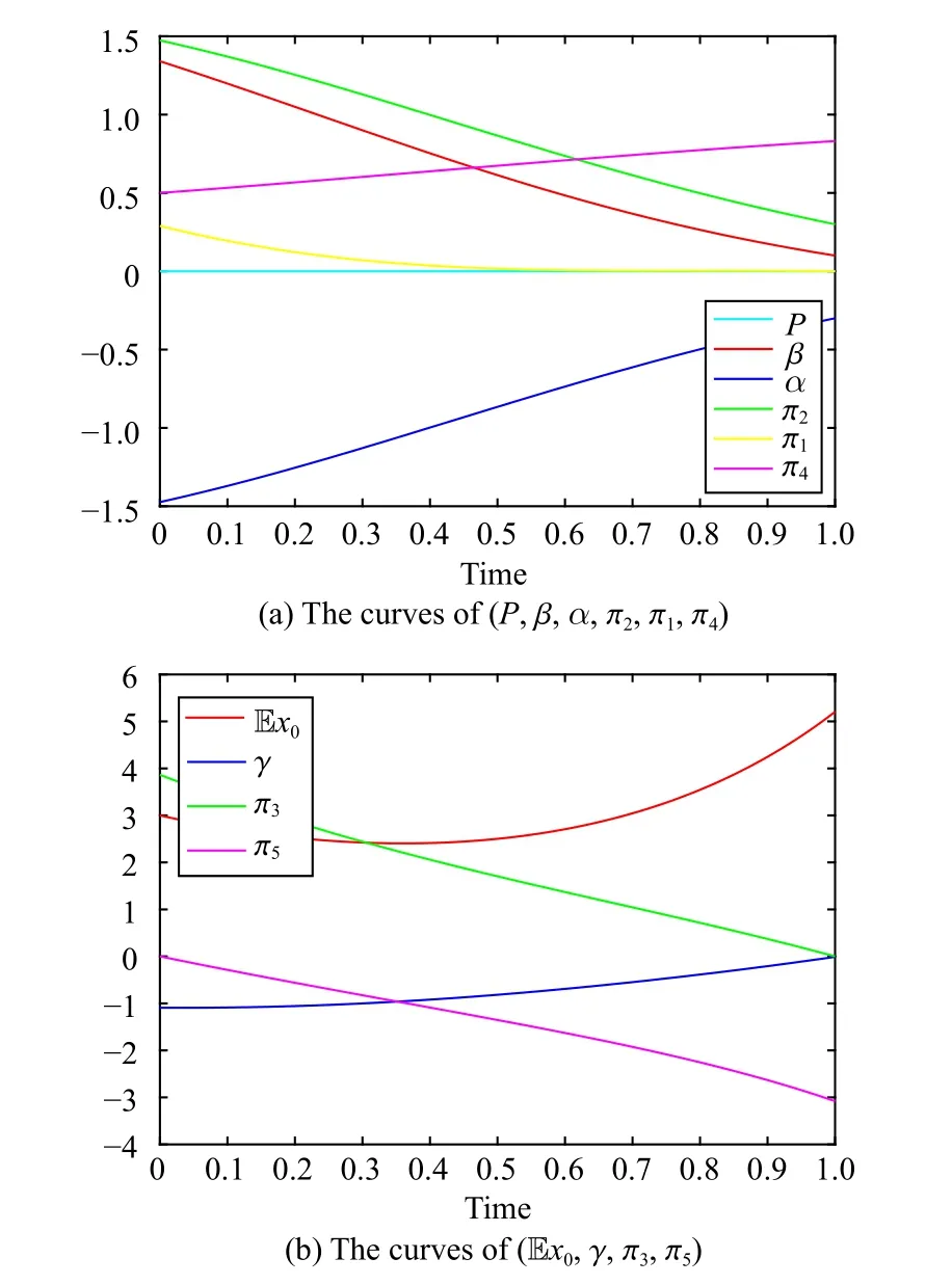
Fig.3.Numerical solutions of ( P,β,α,π2,π1,π4) and ( Ex0,γ,π3,π5).

Fig.4.Numerical solution of u *i ( 1 ≤i ≤100).

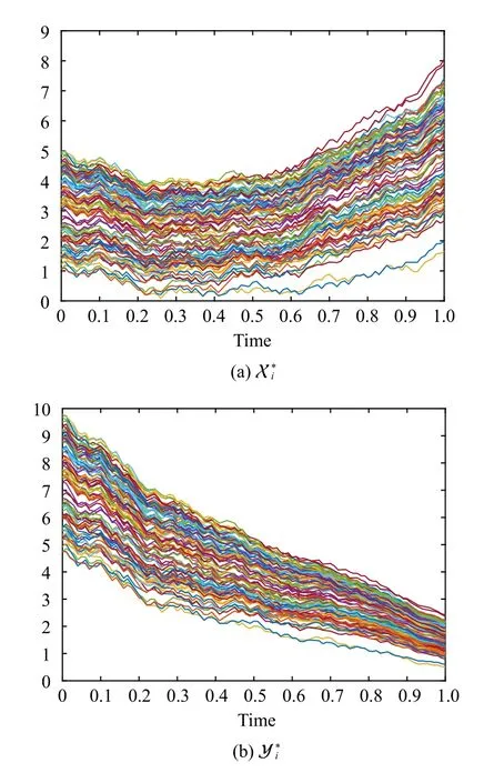
Fig.5.Numerical solutions of X *i and Y *i ( 1 ≤i ≤100).

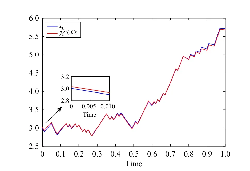
Fig.6.Numerical solutions of x0 and X *(100).

VI.CONCLUSION AND OUTLOOK

This paper discusses a mean-field game of FBSDE in the framework of partial observation.Employing the filter technique to solve a limiting control problem, a decentralized control strategy is obtained, which is further verified to be anϵ-Nash equilibrium of mean-field game.We also show a financial example with some numerical results.

Wepointoutthat the results established inthisworkare basedonDefinition 1,where theadmissiblecontrol setU¯iobserved by all agents.That is to say,Wis absent from U¯i,depends on the common noiseW.In reality,Wmay not be which results in the unavailability of Lemma 1.In this case,how to solve Problem II will face many technical challenges.We will come back to this topic in our future work.

APPENDIX A PROOF OF LEMMA 1

Proof: Set

whereINand 1N×NrepresentN×Nidentity matrix andN×Nmatrix with all entries equal to 1, respectively.Then the first equation of (1) is

APPENDIX C PROOF OF THEOREM 1

Proof: i) Noting the fourth equality of (18), we assume that

APPENDIX D PROOF OF LEMMA 4

To prove Lemma 4, we first present a lemma (Lemma B1).Let

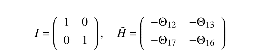
and let 0 be a zero matrix (or vector).Introduce

Inspired by Theorem 5.12 in [39], we introduce

whose unique solution is

Lemma B1: Under Assumptions 1-3, (70) and (71) admit unique solutions.

Proof of Lemma B1:LetP˜=VU-1, which satisfies

Then (70) is solvable.Assume thatP˜1,P˜2are two solutions of (70).SetPˆ˜=P˜1-P˜2.ThenPˆ˜ satisfies

Gronwall’s inequality impliesPˆ˜ ≡0.This proves the uniqueness for (70).Hence, (70) is uniquely solvable.Based on this, (71) is uniquely solvable.■

Proof of Lemma 4: With the above notations, (22), (25),(28) and (35) are written as

Consider

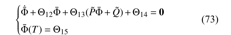
whereP˜ andQ˜ are given by (70) and (71).Then (73) admits a unique solution Φ¯.Define ϕ ¯=P˜Φ¯+Q˜.Then ϕ¯ satisfies

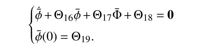
Thus, our claims follow.■

APPENDIX E PROOF OF LEMMA 5

Proof: It follows from (34) that:

Herecrepresents a constant independent ofN.Similarly, we get

and

Based on (74)-(76), we derive

APPENDIX F PROOF OF LEMMA 6

Proof: By (36)-(38), we get

and

Recalling (34), it yields that

and

Taking squares and mathematical expectations on both sides of (77)-(79) in integral forms, we arrive at

where

It follows from Gronwall’s inequality and (80)-(83) that(39)-(41) hold.■

APPENDIX G PROOF OF LEMMA 7

Proof: In accordance with (36) and (37), we get

It follows from (84) and Gronwall’s inequality that (42)holds.Applying some estimate techniques of BSDE to (85),we obtain

Since

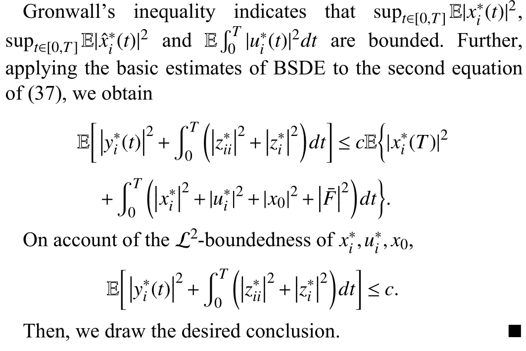
Gronwall’s inequality suggests that

APPENDIX H PROOF OF LEMMA 8

Proof:

wherei∈N.Utilizing (39) and (42) with Hölder’s inequality,we have

Evidently,

Similarly, (42) and (43) imply

Based on (86)-(88), our result holds.

APPENDIX I PROOF OF LEMMA 9

Proof: It follows from the first equations of (49) and (50)that:

and

wherei,j∈N,j≠i.Then we obtain

By the L2- boundedness ofx0,ui,u*j(j≠i) and Gronwall’s inequality, we arrive at