Effects of turbulence models on the numerical simulation of nozzle jets

TANG Zhi-gong,LIU Gang,MOU Bin,H UANG Yong

(1.Northwestern Ploytechnical University,Xi'an 710072,China;2.China Aerodynamic Research and Development Center,Mianyang 621000,China)

0 Introduction

Modern combat aircraft has a large flight envelope,which comprises all kinds of flight status such as low-speed take-off and landing,transonic or supersonic cruise and various maneuvers.Each flight status corresponds to different operation of tail nozzle,where the discrepancy in internal flows may introduce important variation on thrust.At the same time,nozzle jet interacts with the flow around the aircraft's after-body,which has a significant effect on the aerodynamic performance,especially on the drag.Accordingly,simulation for nozzle jet with high fidelity and accurate prediction it's effect on aerodynamic forces are crucial issues in the design of modern aircraft.

It is difficult for current wind tunnel experiment to investigate the interference phenomena of nozzle jet with external flows because all similarity parameters are hard to be satisfied simultaneously.Experiments for forces measure and jet simulation are usually conducted separately,and special afterbody models are needed for jet testing.On the other aspect,to study jet flows using CFD simulation,there is no need for model fabrication,and jet parameters can be set freely.Compared with wind tunnel testing,the numerical method is more efficient and economical.But numerical simulations are always more doubtable than wind tunnel experiments,the numerical accuracy is dependent on the mesh and turbulence models.Thus careful verification and validation are necessary for CFD before it is applied to simulate nozzle jet flows.

Verification and validation of numerical methods is one of the most important subjects in CFD fields.The AIAA drag prediction workshop,for example,as an influential effort has undergone three cycles so far,in which considerable practice guides has been summarized.Similar special workshop has also been constituted in NASA for simulation of flow control.Although there are many investigations on jet flow and it's interaction with aircraft's after-body,but on the point of validation,lots of works are needed to be done to achieve high reliability of numerical methods[1].

Numerical simulation of three kinds of simplified nozzle jet flows are presented in the paper,which are characterized by internal flows internal and external mixing and after-body interference.Take account of practical application,the fully three-dimensional simulation were performed for these flows with the Reynolds averaged Navier-Stokes equations,though they are all axisymmetrical.Then two representative turbulence models(the S-A and the k-ωSST model)and their compressibility corrections were evaluated by comparison with experimental data.Based on these work,which turbulence model should be adopted for numerical simulation of nozzle jet flows are suggested in the conclusions.

1 Numerical Methods

The non-dimensional three-dimensional Reynolds Averaged Navier-Stokes(RANS)in conservation form with the Cartesian coordinates can be written as

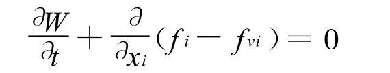
in which the state vector W is[ρ ρ u1ρ u2ρ u3e]T,the inviscid and viscous fluxes vector are

where Reais the Reynolds number calculated with the sonic speed a.

To close the equations,the equation of state for calorically perfect gas,the turbulence model and the Fourier's law of heat conduction are required.The definition of viscous stresses for Newtonian fluid and the Sutherland formula can refer to Ref.[2]in detail.

The in-house RANS solver MBNS3D was adopted to perform current investigation,which is characterized by:

(1)Cell centered finite volume method;

(2)Roe Scheme with the Van Albada limiter and the three-order MUSCL interpolation,HCL entropy fixing;

(3)One-and Two-equation turbulence(the SA,and the k-ω SST)model;

(4)Dual time stepping;

(5)Detached eddy simulation(DES)based on the S-A model;

(6)Parallel computation based on the MPI environment.

Application of turbulence models is the focus of this work.There are five models be employed to evaluate their effects on nozzle flows,which are the S-A turbulence model and its two derivatives,i.e.compressibility correction scheme and DES scheme,the k-ωSST turbulence model and its compressibility correction scheme.These models are designated as SA,SACC,SADES,SST and SSTCC separately in this paper.

The S-A model equation is constructed using empiricism and dimensional analysis[3],with which good results has been achieved in aeronautical applications,but its behavior in jet flows is little known,the purpose of the present study is to review its performance in the free-shear flow s.The non-dimensional S-A model is

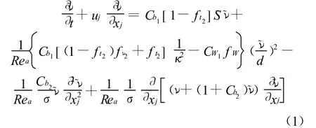
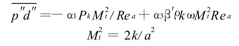
Compressibility correction in supersonic regime is required because the S-A model is developed on incompressible flows;this can be done with addition of a destruction term to the right side of Eq.(1)as follows:

Detached eddy simulation can be implemented with the S-A turbulence model;what need to do is changing the distance function d as～d(Eq.(2)),and then unsteady computation is carried out using the same model equations.

In the Eq.(2),symbol Δstands for the largest distance between current cell center and neighbor cell centers,and constant Cdesequals 0.65.In the wall regions,the wall nearest distances is not changed,i.ebecause mesh aspect ratios can be as much as 1000 times.In the region depart from walls,there isCdesΔ,the S-A turbulence model can switch to a SGS type eddy viscosity model due to

Great progresses in DES have been achieved so far,some convincing simulations are reported about flows around airfoil,delta-wing,fore-body and the F-16 aircraft etc.It can be seen from the Eq.(2)that the wall distance are correlated with meshing,i.e.the longitudinal and lateral grid density both decide the turbulence parameter,so DES is affected much by meshing.In addition,DES is time consuming because of unsteady computation;parallel techniques are needed for complicated geometries.

As another common turbulence model utilized in engineering applications,the Menter's k-ωSST two-equation turbulence model was developed by combination of the k-εand the k-ω models with a blending function.It can be utilized to simulate small separated flows.Its non-dimensional form which includes compressibility correction term can be formulated as follows

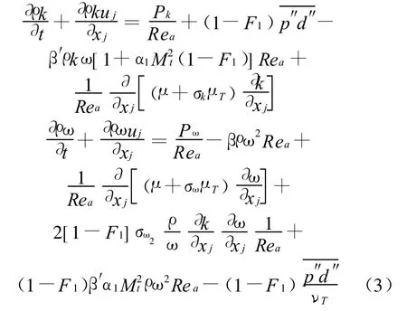
where the pressure shift term is

In order to simulate jet flows,some special boundary conditions are required,which include:

(1)Engine inflow boundary condition.Total temperature and total pressure are specified,and then the Mach number and flow direction on the boundary can be extrapolated with following relations.

(2)Pressure outlet boundary conditions.The value of static pressure is specified when the flow is subsonic.All other flow quantities are extrapolated from the interior information.

(3)Wall boundary conditions.In viscous flows,the no-slip boundary condition is enforced at walls by default.

2 Results and Discussion

Three test examples of nozzle jet flows are studied as follows.

2.1 Supersonic axisymmetrical nozzle

This nozzle model is an axisymmetric,converging-diverging nozzle designed and studied by J.M.Eggers in 1962,in which the air is utilized as working fluid and is operated at the pressure ratio corresponding to perfect expansion.Jet exit Mach number of this nozzle is 2.2.Velocity profiles and eddy viscosity distributions within the jet are delivered by NPARC alliance for validation.

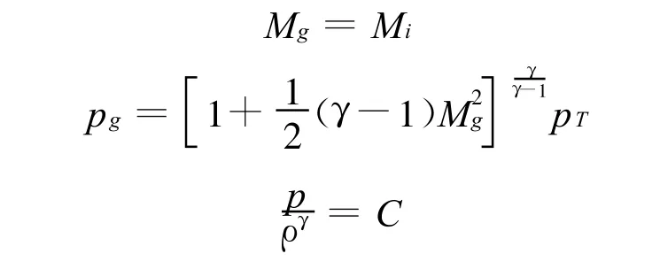
Viscous wall boundaries are specified on the internal nozzle surfaces while inviscid ones are specified on the external nozzle surfaces,since the influence of the exterior boundary layer is not considered significant for this analysis.Fig.1 shows the schematic of grids,which are refined in the interior regions of the nozzle,especially in region adjacent to the walls.Far-field boundaries are as far as 50 times the diameter of the nozzle exit.The circumferential angle of the grid is 180°,and the circumferential boundary are specified as symmetrical boundary conditions.T he angle might be smaller,it was suggested that the grid dimensions should be greater than or equal to three to ensure interpolation at cell surfaces with accuracy of two-order.

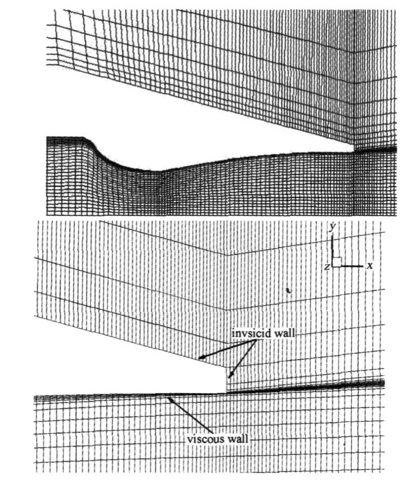
Fig.1 Grid of axisymmetric nozzle图1 轴对称喷管计算网格

Computation was performed using the LU-SGS implicit time-marching approach of the MBNS3D to achieve a steady-state solution.Local time step-size at each iteration was adopted to accelerate the timemarching process until the convergence criterion is achieved as Fig.2 shown.

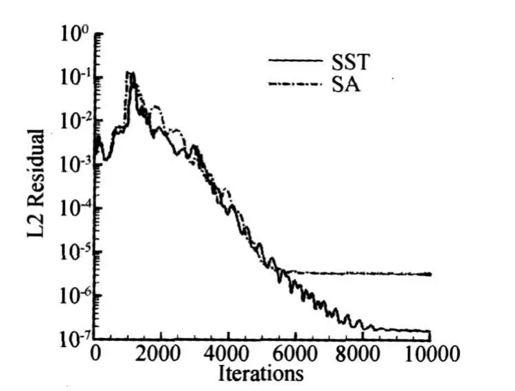
Fig.2 History of residual value(Ma=0.05)图2 残值收敛历程(Ma=0.05)

The incoming flow conditions include Mach number Ma=0.05,the static pressure P∞=1.014×105Pa,and the static temperature T∞=292K.The stagnation conditions of the combustion chamber include that the total pressure P0=1.118×106Pa and total temperature T0=292K.The nozzle pressure ratio is NPR=11.034,it corresponds to a perfect expansion and an exit Mach number of 2.22.The Reynolds number calculated with one foot and sonic speed equals 7.88×107.If the free-stream Mach number is specified to 0 at the lateral far-field boundaries that is not far enough,numerical simulating will produce unphysical phenomena such as asymmetrical jet due to the lack of algorithmic symmetry.Then a tiny value of free-stream Mach number(Ma=0.05 in this case)is set at these boundaries to exclude this anomaly.

The histories of residual value in simulation with the SA model and the SST model are shown in Fig.2;the SST model corresponds to a better convergence which can reach the machine 0 after 10000 iterations.Detached eddy simulation based on the SA model was performed by dual-time stepping method,whose time interval equals 0.005 and the inner iteration of 5 steps make the residual decrease by 1/10.

Contours of Mach number and eddy viscosity computed by the SST model and its compressibility correction scheme are compared in Fig.3 and Fig.4,it can be seen that the maximum eddy viscosity drop by 5000 with the compressibility correction scheme,in which the jet's diffusion rate is reduced greatly.

The axial velocity is scaled by the reference axial velocity(538.32m/s).T he axial distance is the distance from the nozzle exit scaled by the nozzle exit radius(0.0128m).Then the velocities along the centerline are shown in Fig.5.It appears that the accuracy of these computations is sensitive to the modeling for turbulent flow;axial velocities predicted with the SA model and the SST model are spread out at a greater rate than predicted in the experiment.Results of SACC,SSTCC and SADES are close to the experimental data,among which the data of SSTCC have good agreement along all the centerline,the data of SACC only at the first half part,and the data of SADES are greater than the experimental value due to less diffusion.

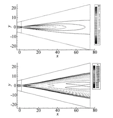
Fig.3 Mach and eddy viscosity contours(SST model)图3 马赫数和涡团粘性系数等值线(SST模型)

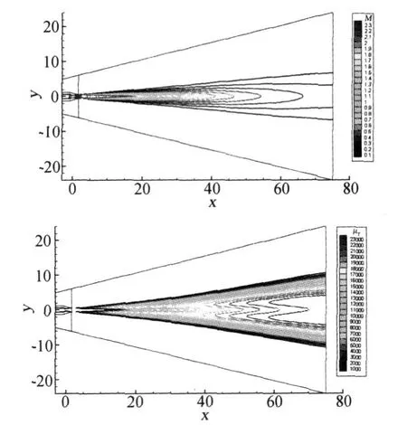
Fig.4 Mach and eddy viscosity contours(SS TCCmodel)图4 马赫数和涡团粘性系数等值线(SSTCC模型)

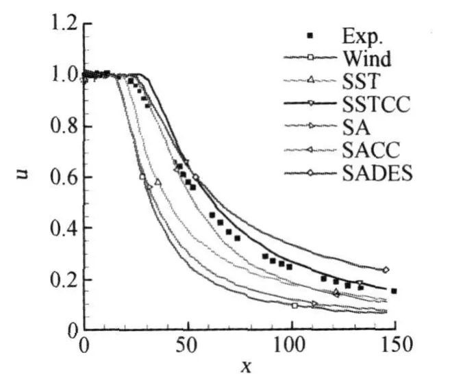
Fig.5 Comparison of velocities along the centerline图5 中心线上喷流速度比较

The jet velocity profiles in the radial direction at several axial stations downstream of the nozzle exit were examined and compared to the experimental values in Fig.6.These comparisons were made at five axial stations,i.e.x=0.0,26.93,51.96,73.80,and 121.30,which are distances from the nozzle exit nondimensionalized by the nozzle exit radius.It appears that data of SSTCC are in good accordance with the measured results at all stations,the data of SACC are good only at first two stations,but not at last three stations.The accordance of the results from SADES with experimental values is achieved at first three stations,and then the accuracy is reduced at last two stations.This deviation might be caused by coarsen grids at downstream fowfield,which can't fulfill requirements from the Detached Eddy Simulation.

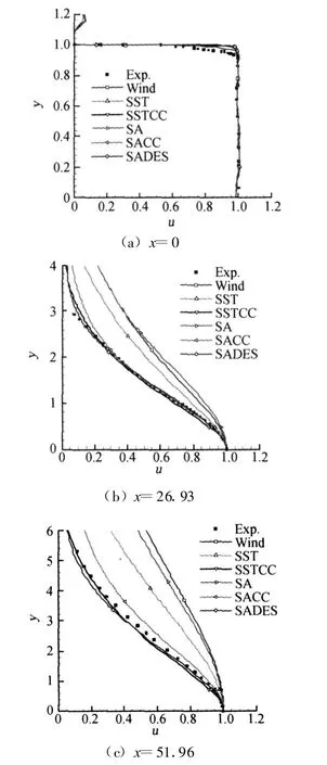
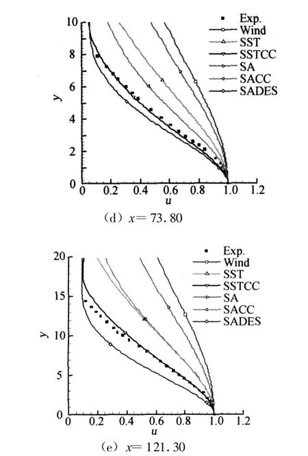
Fig.6 Comparison of velocity profiles图6 速度型比较

2.2 NASA D-1.22-L boat tail/nozzle configuration

In this case,the NASA D-1.22-L boat-tail/nozzle configuration documented in NASA TP 1766 is simulated.Computational conditions include the nozzle pressure ratio(NPR)of 1.5,the free stream total pressure of 1.014×105Pa,the free stream total temperature of 329K,the free stream Mach Number of 0.8,and the nozzle total pressure of 0.998×105Pa.The unit Reynolds number is 1.2×107/m.

Fig.7 shows the multi-block abutting grids of the test configuration,in which wall boundaries are set to viscous adiabatic boundaries.The interactions between internal and external flows must be predicted in this case;therefore mesh lines are gathered together at the nozzle exit.Fig.8 shows the pressure contours in the flow field,where smooth pressure distribution can be discerned around the tail.The predicted pressure coefficients are compared with test data and other referenced data in Fig.9;it shows that present results are in good agreement with the experimental data.The external wall surface pressures obtained with different turbulence models have no difference with each other as shown in Fig.10.

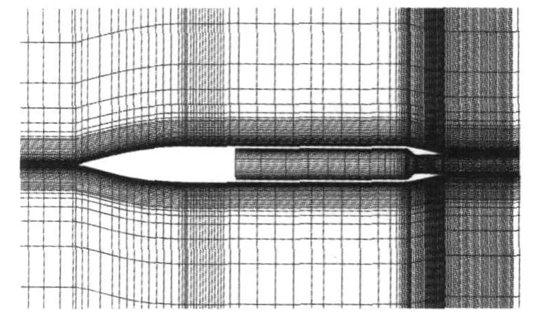
Fig.7 Grids of NASA D-1.22-L boat tail/nozzle configuration图7 NASA D-1.22-L船尾/喷管构型网格

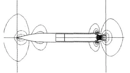
Fig.8 Pressure contours图8 压力等值线

Fig.9 Comparison of pressure coefficients图9 压力系数比较

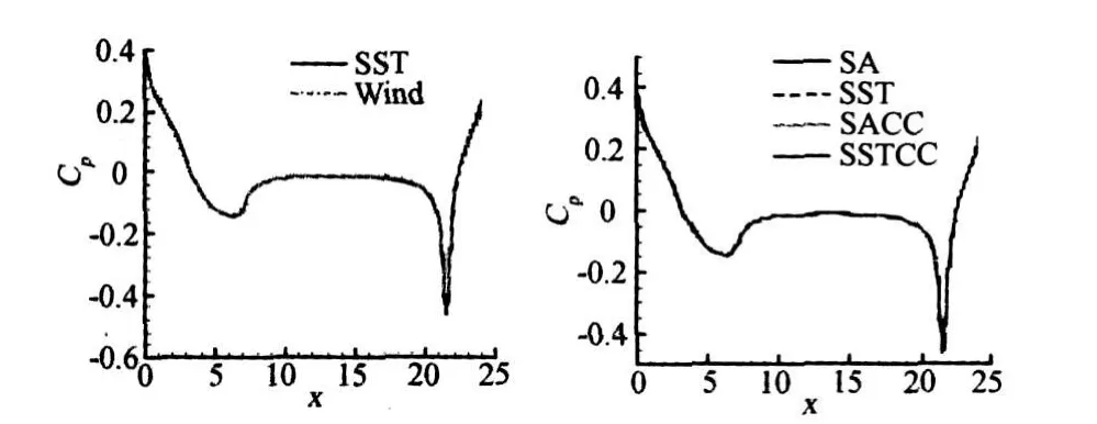
Fig.10 Pressure coefficients of different turbulence models图10 不同湍流模型的压力系数

2.3 Axisymmetric circular-arc boat tail nozzle

The nozzle configuration and experimental data are selected from reference[11-12].This case correspond to transonic flight status with shock-induced separations and strong adverse pressure gradients,which challenge the CFD code to the simula-tion ofexternalafter-body and internal nozzle flows.Fig.11 show s the schematic of nozzle geometry.The flow conditions of free stream and nozzle inflow are listed in Table.1 at the nozzle pressure ratio of 21.23.

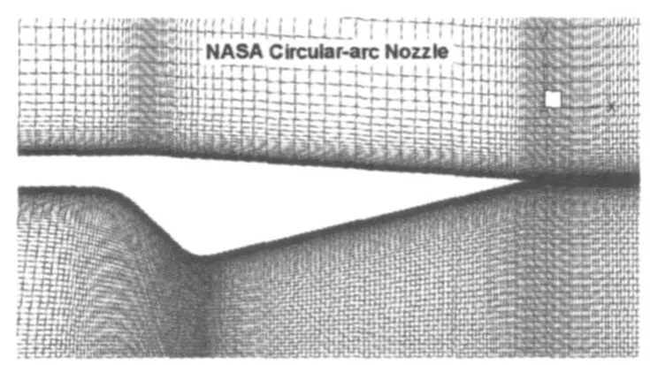
Fig.11 Schematic of nozzle geometry图11 喷管外形及网格

Table 1 Flow conditions(NPR=21.23)表1 流动条件(NPR=21.23)

At the design point(NPR=21.23),the simulated flow field is shown in Fig.12.Flow is accelerated to supersonic speed through the nozzle,and then a sophisticated array of shocks and expansion waves is formed.The wave structures are described richly and clearly,which testify to the accuracy of current methods to some extent.

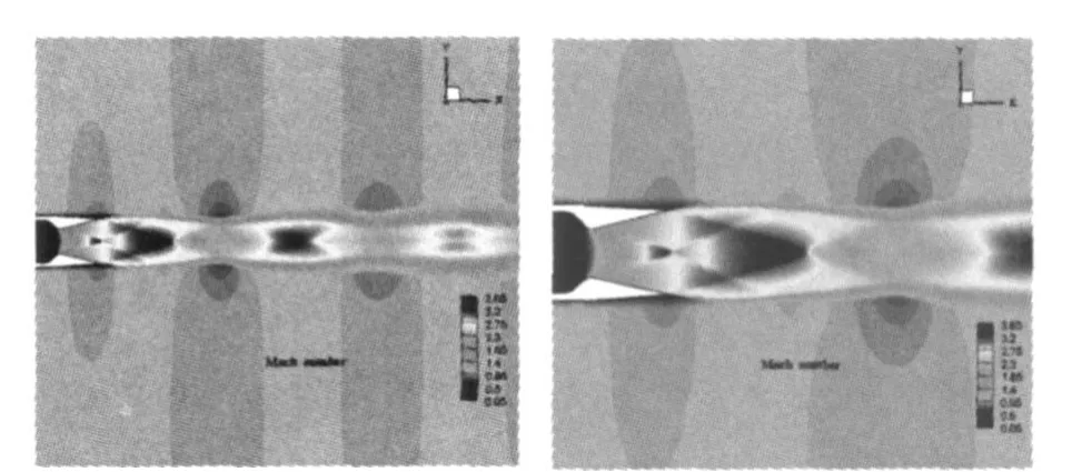
Fig.12 Mach number contours(NPR=21.23)图12 马赫数等值线(NPR=21.23)

Off-design nozzle performance is simulated at Ma=0.9 and NPR=4,the pressure distribution on the external and internal surfaces are shown in Fig.13 and Fig.14.It appears in Fig.13 that the external wall pressure coefficients calculated with four turbulence models all agree well with the experimental data,however there are small differences when x/D＞0.45,where internal separated flows take effect.It can be seen in Fig.14 that flow separate at x/D=0.75,the SST turbulence model predicts the position nicely,and has the best agreement with the experimental data on internal and external pressure distributions.The predicted separation of SA turbulence model lags,but the pressures in separated region are close to the experimental data.All compressibility correction schemes cause the separation to move upstream and the wall pressures in the separated region are overestimated comparing with the experimental data,which disturb the external pressure distribution at the same time.

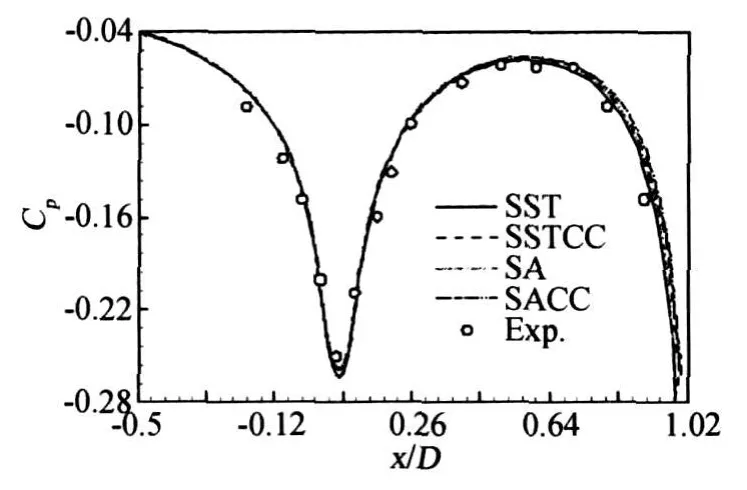
Fig.13 Cpvalues on the external surface图13 尾喷管外表面压力系数

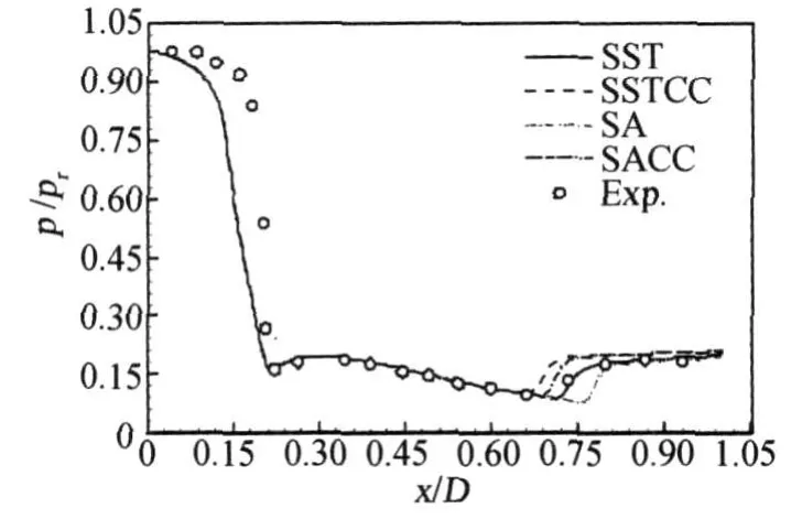
Fig.14 Pressure distribution on the internal surface图14 喷管内表面压力分布

Fig.15 shows Mach number contours of different turbulence models,it appears that the compressibility correction schemes bend the shock lines in the center,and the low-speed region close to the exit is expanded.Wave structures of each turbulence model are similar to the other,main differences lie on the shape of the centered normal shock and its induced vortex.Fig.16 shows the streamlines and Mach number contours calculated with the SST compressibility correction scheme,typical vortex structure can be seen behind the normal shock.This phenomenon can be explained with less numerical diffusion;in other words,the eddy viscosity may be reduced substantially by the compressibility correction schemes.

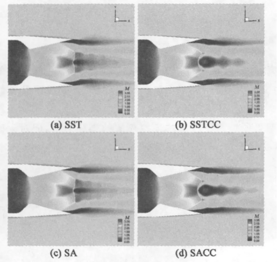
Fig.15 Effects of turbulence models图15 湍流模型的影响

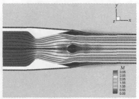
Fig.16 Streamlines and Mach number contours simulated with compressibility correction scheme图16 湍流模型考虑可压缩修正得到的流线和马赫数云图

3 Conclusions

CFD analyses for three test cases have been performed to better understand the validity of the MBNS3D code on simulation about the nozzle jet flows.Flow phenomena such as boundary layer separation and shock wave/boundary layer interaction complicate the implementation of numerical simulation.Diversities in results obtained with four different turbulence models have been presented in this paper.The Compressibility correction schemes improve greatly the trends of jet expansion,the separation locations predicted with this correction,however don't agree so well as their original models.In nozzle flow simulations,better agreement with experimental data can be obtained with the k-ωSST model and its compressibility correction,and the advantage of the S-A detached eddy simulation is not remarkable on the same grid compared simulation with the S-A model.

[1]NORTH ATLANTIC TREATY ORGANIZATION.Aerodynamics of 3-D aircraft afterbody[R].Agard Advisory Report No.318,Sept.1995.

[2]MOU Bin.Numerical simulation and investigation of flow control[D].China Aerodynamics Research and Development Center Graduate School,2006.(in Chinese)

[3]SPALART P,ALLMARAS S.A one-equation turbulence model for aerodynamic flows[R].AIAA 92-0439,1992.

[4]SPALART P R.Trends in turbulence treatments[R].AIAA 00-2306,2000.

[5]FORSYT HE J R,HOFFMANN K.A detached-eddy simulation with compressibility corrections applied to a supersonic axisymmetric base flow[R].AIAA 02-0586,2002.

[6]MENTER F.Zonal two equation turbulence models for aerodynamic flows[R].AIAA 93-2906,1993.

[7]FORSYTHE J R,HOFFMANN K A,SUZEN Y B.Investigation of modified Menter's two-equation turbulence models for supersonic applications[R].AIAA 99-0873,January 1999.

[8]FORSYTHE J R.Numerical computation of turbulent separated supersonic flow fields[D].[PhD.Dissertation].Aerosp.Eng.,Wichita State U.,Spring 2000.

[9]EGGERS J M.Velocity profiles and eddy viscosity distributions downstream of a Mach 2.22 nozzle exhausting to quiescent air[R].NASA TN D-3601,September 1966.

[10]BOBBY L BERRIER,RICHARD J RE.Investigation of convergent-divergent nozzles applicable to reducedpower supersonic cruise aircraft[R].NASA TP-1766,December 1980.

[11]CARSON G T JR,LEE E E JR.Experimental and analytical investigation of axisymmetric supersonic cruise nozzle geometry at Mach numbers from 0.60 to 1.30[R].NASA TP-1953.

[12]TERYN DALBELLO,NICHOLAS GEORGIADIS,DENNIS YODER.Computational study of axisymmetric offdesign nozzle flows[R].AIAA 2004-0530/NASA TM 2003-212876.