Determination of seepage velocity in streambed using temperature record of Russian River, USA*

WU Zhi-wei (吴志伟), SONG Han-zhou (宋汉周), HUO Ji-xiang (霍吉祥)

College of Earth Science and Engineering, Hohai University, Nanjing 210098, China, E-mail: wzw85@126.com

Determination of seepage velocity in streambed using temperature record of Russian River, USA*

WU Zhi-wei (吴志伟), SONG Han-zhou (宋汉周), HUO Ji-xiang (霍吉祥)

College of Earth Science and Engineering, Hohai University, Nanjing 210098, China, E-mail: wzw85@126.com

(Received October 4, 2012, Revised April 7, 2013)

The vertical seepage velocity is an important parameter in the groundwater-surface water (GW-SW) exchange process. It is reported that the periodical fluctuated temperature record of the streambed can be used to determine the seepage velocity. Based on a 1-D flow and heat transport model with a sinusoidal temperature oscillation at the upstream boundary, a new analytical model is built. This analytical model can be used to determine the seepage velocity from the amplitude ratio of the deep and shallow test points. The process of calculation is discussed. The field data are superimposed by multi-periods, so the spectrum analysis and the data filtering are desirable. For the typical seepage medium, the analytical model is effective to compute the seepage velocity between –2 m/d and 6 m/d by using the record of the daily period fluctuation. The temperature time-series analytical model is used to determine the upwards seepage under the condition that the spacing of test points is small (less than 0.2 m). Lastly, a case study for the Russian River shows that this model is very convenient to determine the temporal changes of the GW-SW exchange.

temperature record, groundwater-surface water (GW-SW) exchange, streambed, analytical model, Russian River

Introduction

The groundwater and surface water exchange (GW-SW exchange) plays an important role in many fields, such as the hydrogeology, the hydrology, the environmental science and the water resource management[1,2]. But the rates of the GW-SW exchange and the properties of the streambed permeability medium have temporal and spatial variations, which are influenced by the surface water dynamics, the geological conditions and other external factors. The temporal and spatial variations of the GW-SW exchange are very complex and were also much studied. It was suggested that the heat provides a natural tracer for tracing the groundwater movement[3,4]. For the stream flow, the streambed temperature record can be used to determine the temporal and spatial variations of the GW-SW exchange[5,6].

The water between a stream and adjacent sediments carries a measurable amount of heat. The GW-SW exchange patterns can be inferred qualitatively based on the variations of the streambed temperature data. The early qualitative studies include the simultaneous analysis of the streambed temperature and the stream flow patterns, or the analysis of the temperature anomalies (thermal-pulse) and the temperature envelopes. From these analyses, the flow state of the groundwater, i.e. the discharge or the recharge, can be determined[7,8]. At the same time, there were some modeling studies of the groundwater flow with heat transfer. Most of the models are based on the heat advection and conduction in geological media. The upper boundary temperature is often assumed to be in a sinusoidal fluctuation. Such an assumption has a sufficient reliability in the study of the seepage velocity. These heat transfer models may be used to numerically inverse the GW-SW exchange by the streambed timeseries temperature data. If the observational stream temperature is taken as a model input, the inversion results will be more accurate[9].

Influenced by the steam flow, the streambed temperature fluctuates periodicity. And the periodical fluctuation is closely related with the GW-SW exchange rate. Compared with the stream temperature, the mea-sured time series data of the streambed temperature show a damping in the amplitude and a phase lagging. And this change is mainly governed by the groundwater seepage velocity and the depth of the test points. The analytical solution of the time series data can be used to inverse the groundwater-surface water exchange rate. Providing that the stream temperature varies sinusoidally, the vertical seepage velocity can be obtained by an analysis model based on the amplitude damping or the phase lagging. The well-known studies include those by Hatch et al.[10]and Keery et al.[11]. Compared with the Hatch model, the Keery model does not take the thermal dispersivity into account. Some follow-up studies have discussed the shortcomings of Keery and Hatch models[12].

The uncertainty of the analytical model can be evaluated by a numerical modeling[13]or sand box experiments[14]. It is shown that the calculated velocities are sensitive to the thermal properties of the saturated sediment and to the spacing between test points, but insensitive to the thermal dispersivity. Some studies suggest that the amplitude ratio is not sensitive to the thermal skin effect (TSE), for the temperature measured inside a pipe buried in the sediment[15]. But the phase lagging is very sensitive to the TSE.

A variety of methods were reported to isolate the daily signals from the measured temperature. Hatch et al.[10,16]isolated the signals using a cosine taper bandpass filter. Keery et al.[11]isolated the signals using a Dynamic Harmonic Regression (DHR) filter. And Gordon et al.[17]developed a computer program named VFLUX to calculate the vertical flux from the field temperature time series automatically. This program is based on the DHR method. In fact, the instantaneous or the gradual changes in the flux over time can also be captured by a one-dimensional heat transport model[18].

This paper proposes a new analytical model and describes the calculation process in detail, as how to use the amplitude damping of the time series data to compute the seepage velocity. Then the applicability of the analysis model is discussed. And the data collected from the Russian River (California, USA) are taken as a case study. The site study is to demonstrate the usefulness of the analysis model.

1. Analytical model of temperature time series record

1.1 Temperature as a tracer

The heat advection plays a major role in the heat exchange between the stream and the streambed, that is to say, the heat exchange is governed by the groundwater flow. In most cases, the groundwater vertical movement is the main mode of the GW-SW exchange. So a 1-D heat transfer model is commonly used. If the groundwater keeps still, the lower frequency part of the temperature fluctuation can penetrate into a deeper area. The measured and simulated streambed temperature record indicates that the timeseries records have an obvious daily fluctuation in the shallow streambed. While the seasonal or annual fluctuations are shown in deeper areas, for a losing stream, the oscillating temperature signal near the surface will penetrate deeper than for a non-flow stream. The heat advection will make the temperature peaks to become smaller and the lag shorter than a non-flow stream. For a gaining stream, the surface fluctuation will decline normally or even faster in deep area. deeper points are denoted as Asand Ad, respectively. Then the ratio ofAdand Ascan be correlated with

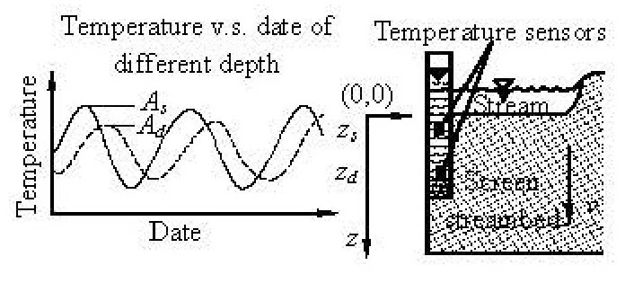
Fig.1 Schematic diagram of using the measured streambed record to trace the groundwater-surface water exchange

The phenomenon mentioned above that the temperature oscillation is governed by the groundwater seepage will provide the basic methodology for the temperature tracing. As shown in Fig.1, the amplitude of the temperature time series data at shallower and the vertical seepage velocity of the streambed.

In the site tests, the sediment temperatures can be measured directly by temperature probes put in the streambed, or indirectly by installing the probes at a certain depth in the observation well. Commonly, the well is cased by plastic or metal pipes. For the latter method, the measured water temperature is lagged and damped compared to the temperature outside of the pipe. This phenomenon is known as the Thermal Skin Effect (TSE). In fact, the amplitude damping is less sensitive to the TSE than the phase lagging[15].

1.2 Analytic model

Firstly, the following conditions are assumed: the top surface of the streambed is a plane, the streambed is a semi-infinite space and filled with a homogeneous porous medium. Under these conditions, the transient one-dimensional heat conduction-advection equation is

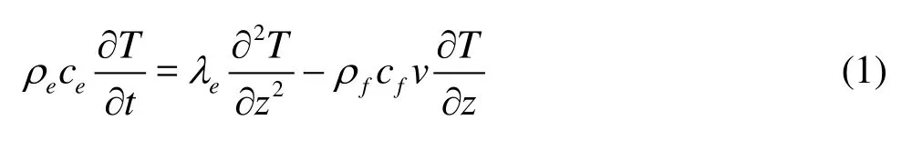
whereT is the temperature at the depthz at the time t,λeis the effective thermal conductivity of the satu-rated sediment,λe=(1-n)λs+nλf, the subscript s represents the solid medium,f represents the fluid, and the thermal dispersivity is ignored,n is the porosity of the porous medium,v is the vertical seepage velocity (positive inz direction, the Darcy velocity), ρeis the effective density of the saturated sediment, ρe=(1-n)ρs+nρf,ceis the effective heat capacity of the saturated sediment,ce=(1-n) cs+ncf.

It is assumed that the temperature of the upper boundary is consistent with the stream temperature and can be described as

where Ais the amplitude of the temperature fluctuation atz =0,P is the period (a day or a year),T0is the non-oscillating part of the temperature, which is equal to the average temperature.

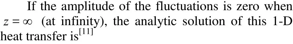
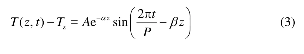
where Tzis the temperature at the depth zand the timet , without the influence of the sinusoidal fluctuation propagated from the surface.αandβare coefficients defined as:

The right side of Eq.(3) is the the temperature fluctuation at the depth z and the time t. It is obviously influenced by the thermal physical parameters of the porous medium and the fluid, the seepage velocity, the boundary temperature fluctuation and other factors. Generally speaking, the temperature records will have an amplitude damping between shallow and deep test points. And the peaks of the temperature curves also have phase shifts. When the velocity of the downward flow is much greater, the amplitude damping is smaller.

It was shown that the flux derived by using the phase shift would involve more errors[19]. So we just consider the amplitude of the time-series record. From Eq.(3), the amplitude of the temperature record at the depthzis

If the amplitude ratio of deeper and shallower points is denoted as Ar,Ar=Ad/As, then

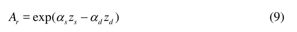
As mentioned previously, the streambed is homogeneous, i.e., the physical properties of the streambed is the same everywhere. From Eqs.(3) and (9), we can obtain the following expression

where Δzis the spacing between shallower and deeper points(Δz= zd-zs). Equation (10) gives the dependencies of the amplitude ratio on the oscillating factor and the average vertical seepage velocity between two points. At a given time, the seepage velocity is constant, so the amplitude ratio is constant. The seepage velocity can be calculated from Eq.(10) at a given time.

Equation (10) can be evaluated by MATLAB®if the amplitude ratio, the test points spacing Δzand the thermal physical parameters are known. The equation may contain some virtual roots. In practical applications, the real root is adopted to represent the average vertical seepage velocity.

In particular, Eq.(10) is based on the assumption that the stream temperature varies sinusoidally. So the measured record should be filtered to obtain the daily or annual fluctuation curves.

1.3 Computing procedures

The procedures of applying the analytical model are as follows:

(1) Recording: Avoid such measured errors as would be caused by external factors such as misoperation.

(2) Spectrum analysis: To find out the vibration frequency of the record by the FFT method. Comparethe energy intensities of the daily, seasonal and annual signals and choose the most significant signals as the basic analysis data.

(3) Digital filtering: The band-pass filters are used to obtain the signal fluctuations with the main period. In fact, most of the streambed temperature records show a significant daily fluctuation feature, because it is convenient measuring the temperature of the shallow area (0 m-3 m). A great amount of effective information can be obtained in short time. So the range between the high-pass and the low-pass can be set to 24 h in a band-pass filter.

(4) Peak extraction: Record the coordinates of extreme points of the filtered temperature record. This can be done by manual or numerical methods. Then the temperatures at extreme points are used to calculate the amplitude ratio Ar.

(5) Compute the seepage velocity: Based on the optimization method in MATLAB®, compute the average vertical seepage velocity between shallower and deeper points from Eq.(10).

(6) Assess the temporal and spatial variabilities of the streambed GW-SW exchange: the results are expressed by a continuous curve of the streambed flow velocity vs. the date. From this curve, the temporal variations of hydrological or hydrogeological conditions will be assessed. And since such analytic method is very easy to use, it is feasible to collect a sufficient number of measuring points. So this method will also be used to assess the spatial permeability.

Table 1 Thermal parameters of typical permeability medium

2. Applicability of analytic method

2.1 Typical permeability medium

Most of the streambed is filled will sand, silt, clay or their combinations. The deposit of the case study (Russian River, CA, USA) that follows is the sand. This paper takes the sedimentary material of the Russian River as a typical permeable medium. The values of some related parameters for the calculation are shown in Table 1. A porosity of 0.370 is chosen as the representative value for the medium sand. The heat capacities and the thermal conductivity values are based on literature values for the sand. The heat capacities and thermal conductivity values for the water are based on empirical values.

2.2 Temperature fluctuation without groundwater influence

If the groundwater keeps still, the amplitude ratio of two points is

As shown in Eq.(11), when the Δzis a constant, the penetrated depth of the periodicity fluctuation factor (denoted here byArat the depth z) is inversely proportional to the density and the heat capacity of the saturated sediment, which is proportional to the period and the thermal conductivity coefficient. The above pattern is also applicable for the streambed with groundwater flows.

Fig.2 Amplitude ratio Arof a given spacing of test points Δz when v =0

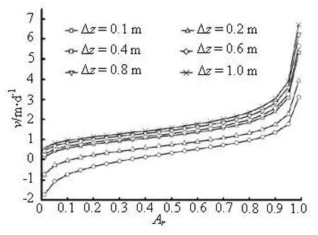
Fig.3 Amplitude ratio Arvs. seepage velocity v at different spacings of test points Δz

For the medium mentioned above, the amplitude ratio Arfor a given spacing of test points Δzis shown in Fig.2.

The amplitude ratio damps exponentially withthe increase of the spacing between points concerned. With the calculated parameters shown in Table 1, the amplitude ratio is close to zero when the spacing of test points is greater than 0.5 m. So when the spacing between two points is too large, the deeper point can not be made visible from the daily fluctuation signals. In the absence of groundwater flow, the heat conduction can only make the temperature fluctuate at a shallow area.

2.3 Applicability of analytic model

For different spacings of test points, the amplitude ratio Arvs. the vertical seepage velocityvis shown in Fig.3.

From Fig.3, It can be seen that:

(1) Compared with the heat conduction, the temperature fluctuation will be penetrated deeper by the fluid flow. For example, when Δz=1.0 m,Aris greater than zero if the seepage velocity is greater than 0.5 m/d. The identifiedArvalues can be used to determine the groundwater velocity. It means that the spacing of probes should be arranged larger in situations with a more rapid groundwater flow.

(2) At a given depth, the amplitude ratio is nonlinearly dependent on the seepage velocity. And Aris greater whenv is greater. This is consistent with the results of the qualitative analysis.

(3) To determine the groundwater flow by using the daily period data, it is more effective to compute the seepage velocity between –2 m/d and 6 m/d. When the spacing of test points is smaller enough (for example, 0.1 m or 0.2 m in this case), the upward flow can be determined by the analytic model.

(4) In the limit cases of Arwhen Aris very large (close to 1.0) or very small (close to 0), the large range of the seepage velocity corresponds to small changes ofAr. In these cases, the accuracy of the analytic model will be reduced.

When the spacing of the measurement points is very large, the seasonal or annual oscillating factor can be adopted to establish a new model. The influence of the thermal parameters of the saturated sediment should also be taken into account when we use this time-series method.

3. A case study

3.1 Russian River, CA, USA

The Russian River is located in northern California, originating in the central Mendocino County, CA and flowing into the Pacific Ocean in the western Sonoma County, CA (Fig.4). The main channel of the Russian River is about 177 km long and flows southward from the original area to Mirabel Park, where the flow direction turns predominantly westward.

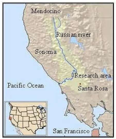
Fig.4 The location of the Russian River and the research area

The Russian River provides a major production and living water for Mendocino, Sonoma, and Marin Counties. The wine industry along the river has continued to increase the demand of the irrigation water. It results in a sustained reduction in the stream water.

The Russian River occupies areas in the northwest of the Santa Rosa Plain, a significant volume of the stream water is exchanged with the alluvial aquifer before the river flows to the west. So the streambed seepage is of particular interest for the water resource management.

The Russian River is underlain primarily by the alluvium and the river channel deposits, which consist mainly of unconsolidated sands and gravels, interbedded with thin layers of silt and clay. The alluvial aquifer is bounded by a metamorphic bedrock, which is considered impermeable.

3.2 Field data

The temperature, the water level elevation, the stage height, and the river discharge data were collected from Hopland to Guerneville, CA over a fouryear period from 1998 to 2002. The observation work was accomplished by the Branch of Regional Research, the USGS, the Western region and Sonoma County Water Agency. In order to illustrate the effectiveness of the analytic method mentioned before, we take the record in Riverfront Regional Park as a case study, which has a more significant daily periodic fluctuation.

For the test points of Riverfront Regional Park, the shallow piezometers were installed in the riverbed sediments using a hand-held casing hammer. The temperature data were collected by the Onset Optic Stowaway data loggers that were hung inside each piezometer at the desirable depth. The depth is about 0.3 m and 0.6 m. An additional logger was hung outside to measure the stream temperature. The loggers recordevery 15 min automatically. The field data from June 19, 2002-September 9, 2002 are shown in Fig.5. 0.6 m logger was lift out of the water after July 25. So the unaccepted records were removed. As shown in Fig.5, the surface stream temperature fluctuates significantly daily. Influenced by the seasonal and hydrological factors, the average temperature is not static. So it can not be described by a sine function directly. The temperatures at deeper points, 0.3 m and 0.6 m, also have daily fluctuations. But their amplitudes vary with time and are always smaller than that of the surface water.

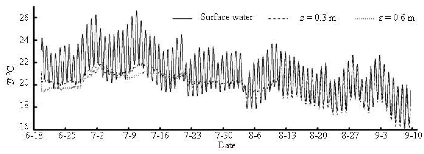
Fig.5 Field temperature records of surface water and streambed

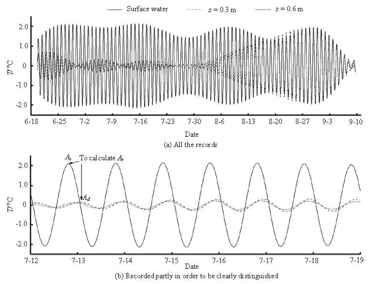
Fig.6 Extracted daily oscillating records

3.3 Extracting daily fluctuation records

The results of spectrum analysis show that the dominant frequency of the field data is 1 d. Therefore theP of Eq.(2) is set as 1 d. That is to say, the daily oscillating data are adopted to compute the groundwater seepage velocity. A band-pass filter with a passband [0.95d,1.05d]is used to process the measured data influenced by multi-periods and multi-factors. Then the extracted oscillating records are shown in Fig.6.

Obviously, the fluctuation factor can be expressed by a typical sine curve with a daily period and fluctuation around zero. The amplitude of deeper one is smaller than shallower one. The time of the appearance of peak points (the maximum or minimum values) lags when compared the shallower and deeper probes. The model input Arcan be obtained from the amplitude of deeper area Adand shallower area As. Since the time lag is very small (less than 1 d), the time when the peak appears at a shallower point is chosen as the model calculating timet . In that case,2(t, Ar)will be obtained daily.

As shown in Fig.6, the amplitude of deeper points is very small in June and July, which indicates that the heat advection is weak. So the measuring point is lightly influenced by the upper temperature fluctuation. But in August and September, the temperature amplitude at point of 0.3 m significantly increases, which indicates that the groundwater activity tends to be stronger than the first two months.

Fig.7 Temporal variability of seepage velocity

3.4 Temporal variability of seepage velocity

From the relevant research literature about this region, the related parameters of the fluid and the sediments are shown in Table 1. Then the analytic model is used to compute the GW-SW exchange velocity. The results are shown in Fig.7. According to Fig.7, the temporal variability of the seepage has the following features:

(1) From June 6-July 25, the flux velocity is small and slightly fluctuating. The velocity is relatively lower at June 29, July 11, and July 25. During this temporal interval, the average seepage velocity in the streambed is 0.36 m/d above 0.3 m and 0.70 m/d above 0.6 m. The comparison between the two timeseries curves shows that their variations are very similar. But the flux in deeper area is stronger than in shallow area, which suggests that the coefficient of the permeability is higher due to the coarser medium.

(2) From July 25-August 15, the seepage velocity increases from 0.02 m/d to 1.59 m/d. During this period, the stream water lever is rising due to rainfall. The high hydraulic gradient will increase the seepage velocity. The average velocity is 0.65 m/d.

(3) From August 15-September 6, the flux is rapid and significantly fluctuating. The velocity curve shows 2 extreme points at August 17 and August 27. This significant fluctuation is related to the stream state when two small-scale floods occurred at that time. The maximum seepage velocity is up to 4.14 m/d. During this period, the average velocity is 2.25 m/d.

(4) Below Wohler Bridge, an inflatable dam acts to increase the river stage during the months of the water demand peak. The back water area results in a higher temperature and lower velocities in the river that extend for approximately 3.2 km. Although the streambed permeability decreases due to the fact that the fine deposition increases, the vertical seepage velocity increases in this case because of the increase of the hydraulic gradient. In the summer, the large agricultural water pumping capacity leads to an increased river recharge to the groundwater.

(5) Some related researches gave the seepage velocity of the Russian river. One of the previous studies shows that the streambed fluxes near Whohler Bridge are near 0.79 m/d-14.03 m/d[20]. And these values are consistent with the results of this paper.

As we have discussed before, the approximate continuous temporal variability of the seepage velocity can be obtained by the temperature time-series analytic method. This method is useful in determining the GW-SW exchange. Based on the site measured time-series records, the temporal variability of the GW-SW exchange rate are easy to be determined.

4. Conclusions

(1) The streambed temperature is affected by the atmosphere temperature. The time-series records have a sinusoidal fluctuation feature. Based on the 1-D heat transfer model in the homogeneous porous medium, an analytical model is proposed to compute the seepage velocity by the amplitude ratio of the oscillating factor. The case study for the Russian River, CA, USA shows that the analytic method is effective.

(2) The use of the analytic method to determine the GW-SW exchange rate should be in the following procedures: process the site record with a band-pass filter to extract the periodic oscillating record, then find the coordinates of peaks and compute the amplitude ratio Arof different points; lastly, compute the seepage velocity.

(3) If the streambed is filled with typical permeability medium, it is more effective to compute the seepage velocity between –2 m/d and 6 m/d from the daily period data. The temperature time-series analytical model can be used to determine the upwards seepage under the condition that the spacing of test points is small (less than 0.2 m).

(4) This analytical model is based on the 1-D heat transfer model. It is applicable to the situation dominated with the vertical seepage. Other methods should be used when the groundwater flows in multidimensions.

Acknowledgments

We also appreciate the information center of U.S. Geological Survey to supply the site measured data.

[1] GRINSVEN M. V., MAYER A. and HUCKINS C. Estimation of streambed groundwater fluxes associated with coaster brook trout spawning habitat[J]. Ground Water, 2012, 50(3): 432-441.

[2] LUO Zhu-jiang, WANG Yan. 3-D variable parameter numerical model for evaluation of he planned exploitable groundwater resource in regional unconsolidated dediments[J]. Journal of Hydrodynamics, 2012, 24(6): 959-968.

[3] ANDERSON M. P. Heat as a ground water tracer[J]. Ground Water, 2005, 43(6): 951-968.

[4] CONSTANTZ J. Heat as a tracer to determine streambed water exchanges[J]. Water Resources Research, 2008, 44(4): W00D10.

[5] NISWONGER R. G., PRUDIC D. E. and FOGG G. E. et al. Method for estimating spatially variable seepage loss and hydraulic conductivity in intermittent and ephemeral streams[J]. Water Resources Research, 2008, 44(5): W05418.

[6] ESSAID H., ZAMORA C. M. and MCCARTHY K. A. et al. Using heat to characterize streambed water flux variability in four stream reaches[J]. Journal of En- vironmental Quality. 2008. 37(3): 1010-1023.

[7] BREWSTER C. J. Delineating and quantifying groundwater discharge zones using streambed temperatures[J]. Ground Water, 2004, 42(2): 243-257.

[8] CHRISTIAN A., KERST B. and RONNY V. et al. A simple thermal mapping method for seasonal spatial patterns of groundwater-surface water interaction[J]. Journal of Hydrology, 2011, 397(1-2): 93-104.

[9] WU Zhi-wei, SONG Han-zhou. Temperature as a groundwater tracer: Advances in theory and methodology[J]. Advances in Water Science, 2011, 22(5): 733- 740(in Chinese).

[10] HATCH C. E., FISHER A. T. and REVENAUGH J. S. et al. Quantifying surface water–groundwater interactions using time series analysis of streambed thermal records: Method development[J]. Water Resources Research, 2006, 42(10): W10410.

[11] KEERY J., BINLEY A. and CROOK N. et al. Temporal and spatial variability of groundwater-surface water fluxes: Development and application of an analytical method using temperature time series[J]. Journal of Hydrology, 2007, 336(1-2): 1-16.

[12] LOPEZ C. D., MEIXNER T. and FERRE T. P. A. Effe- cts of measurement resolution on the analysis of tempe- rature time series for stream-aquifer flux estimation[J]. Water Resources Research, 2011, 47(12): W12602.

[13] SHANAFIELD M., HATCH C. E. and POHLL G. Uncertainty in thermal time series analysis estimates of streambed water flux[J]. Water Resources Research, 2011, 47(3): W035504.

[14] MUNZ M., OSWALD S. E. and SCHMIDT C. Sand box experiments to evaluate the influence of subsurface temperature probe design on temperature based water flux calculation[J]. Hydrology and Earth System Scie- nces, 2011, 15(11): 6155-6197.

[15] CARDENAS M. B. Thermal skin effect of pipes in streambeds and its implications on groundwater flux estimation using diurnal temperature signals[J]. Water Resources Research, 2010, 46(3): W03536.

[16] HATCH C. E., FISHER A. T. and RUEHL C. R. et al. Spatial and temporal variations in streambed hydraulic conductivity quantified with time-series thermal methods[J]. Journal of Hydrology, 2010, 389(3-4): 276-288.

[17] GORDON R. P., LAUTZ L. K. and BRIGGS M. A. et al. Automated calculation of vertical pore-water flux from field temperature time series using the VFLUX method and computer program[J]. Journal of Hydro- logy, 2012, (420-421): 142-158.

[18] LAUTZ L. K. Observing temporal patterns of vertical flux through streambed sediments using time-series analysis of temperature records[J]. Journal of Hydro- logy, 2012, (464-465): 199-215.

[19] LAURA K. L. Impacts of non-ideal field conditions on vertical water velocity estimates from streambed temperature time series[J]. Water Resources Research, 2010, 46(1): W01509.

[20] SU G. W., JASPERSE J. and SEYMOUR D. et al. Estimation of hydraulic conductivity in an alluvial system using temperatures[J]. Ground Water, 2004, 42(6): 890-901.

10.1016/S1001-6058(11)60377-7

* Project supported by the National Natural Science Foundation of China (Grant No. 41272265), the Scientific Research and innovate Foundation to support college graduate of Jiangsu Province (Grant No. CX09B_167Z).

Biography: WU Zhi-wei (1985- ), Male, Ph. D. Candidate

Song Han-zhou, E-mail: songhz@hhu.edu.cn