A Review on Wire Bonding Process in Electronic Manufacturing (PartⅡ)

ZONG Fei, WANG Zhijie, XU Yanbo, YE Dehong, SHU Aipeng, CHEN Quan

（Freescale Semiconductor (China) Limited, Tianjin 300385, China）

3 Phase II - 1st Bonding

3.4 Bonding-1

The bonding-1 phase lasted from the end of the contacting time-1 to the end of the bonding time-1. After this bonding-1 phase the FAB was bonded with the bonding surface and made into a real ball bond finally with the application of USG power (bonding USG-1),force (bonding force-1) and heat (bonding temperature),shown in figure-24.

Although the heat wasn’t the essential factor of wire bonding, increasing bonding temperature did help the bond formation. With the same other bonding parameters,higher bonding temperature got more IMC coverage and relevant higher ball shear strength. The comparisons of IMC coverage and ball shear strength between different bonding temperatures were shown in figure-25 and figure-26 respectively. However, the high bonding temperature could also introduce other issues at the same time, such as risk of initial bond pad cracks, oxidation of bonding surface, evaporation of organics and unexpected IMC phases. Generally, the bonding temperature was set lower than 200 ℃ in the high volume production.

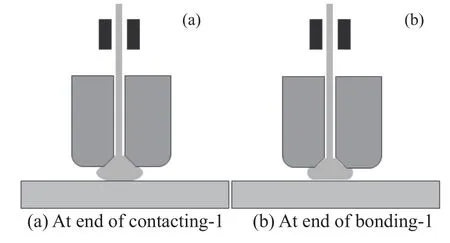
Fig. 24 Sketch of bonding-1 phase

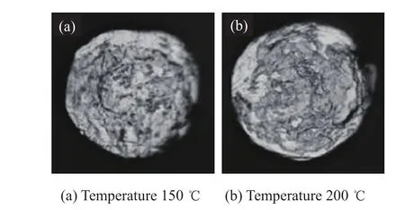
Fig. 25 IMC coverage with different bonding temperatures

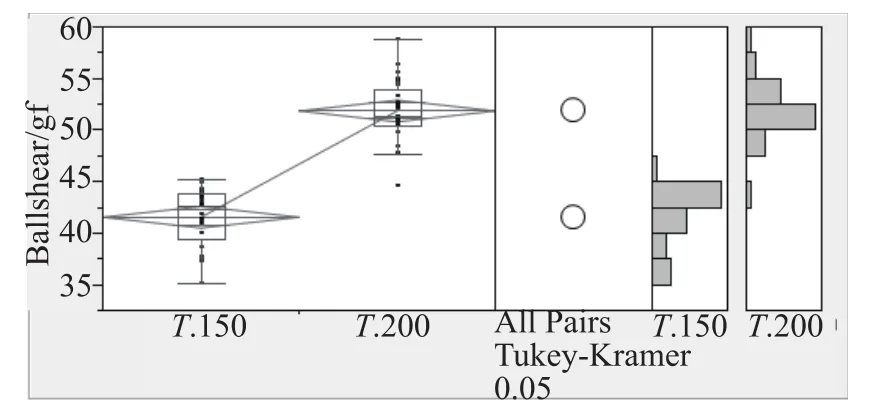
Fig. 26 Comparison of ball shear strength with different bonding temperatures

As discussed above, there was a slipping between the FAB and the bonding surface; and this slipping plays a key role in the formation of micro-weld zones. In fact,the bonding parameters, bonding USG and bonding force,had a great effect on this slipping and the final IMC coverage. Figure-27a[11]showed the stress distribution in the FAB/bond as well as the bonding pad introduced by the bonding force, and the curve was the stress at the bonding interface in Y- direction, σy, whose absolute value was equal to the normal stress, σN. The peaks of normal stress located just below the IC (inner chamfer)zone of capillary. The vibration of bonding USG introduced a tangential force, σf, which was assumed invariable at the interface. Based on the principles of tribology, only when the tangential force was bigger than the product of multiplying the normal force and the friction coefficient, there would be a relative slipping at the interface. In zone-1, the normal force was bigger than the quotient of dividing the tangential force by the friction coefficient, so there wouldn’t the dynamic friction; while in zone-2, the result was opposite and there would be the dynamic friction which would help the formation of IMC and bond. Just as shown in figure-27b[12]. Figure-28 showed the typical IMC distribution at the interface：IMC formed at the centre and the periphery of ball bond (zone 2) and there was a vacancy (zone 1)between them.

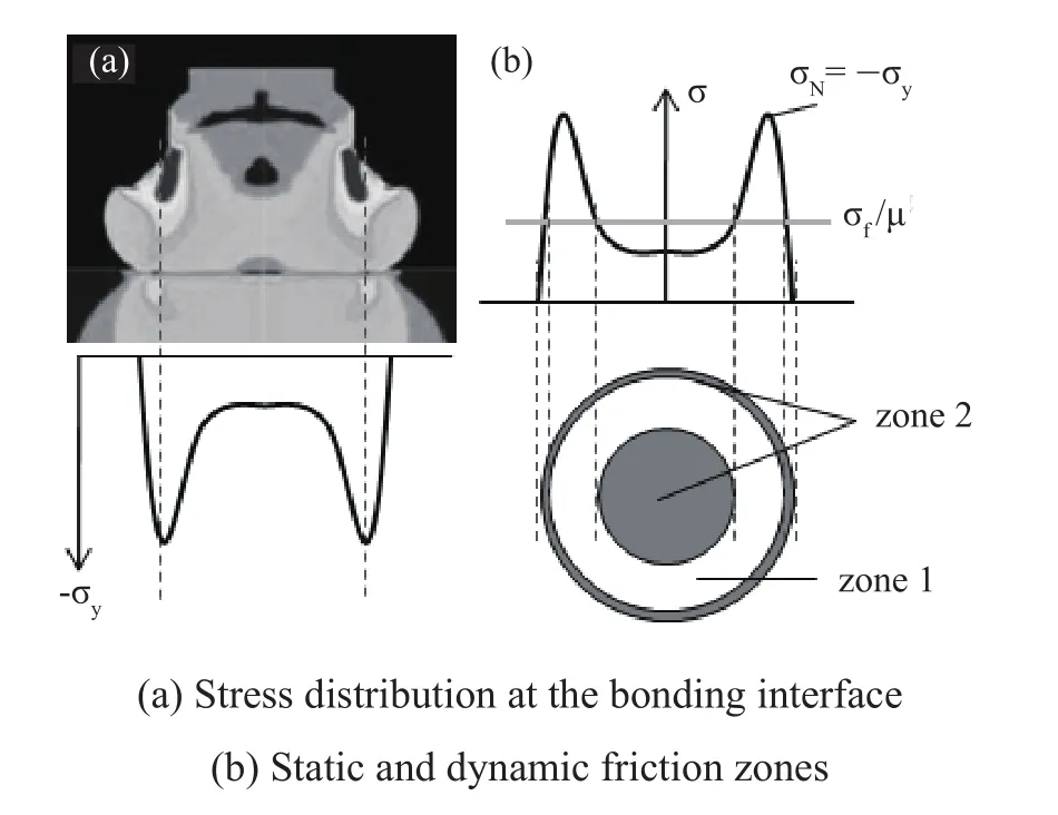
Fig. 27 Interaction between bonding USG and bonding force

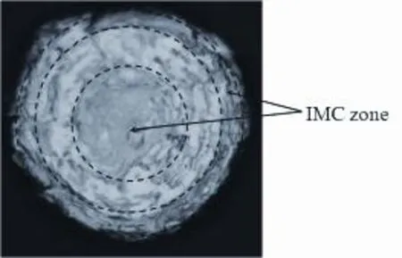
Fig. 28 Typical IMC distribution on 1st bond bottom

Hence if the bonding USG was high while the bonding force was low, the zone-2 would become bigger and more IMC would form at the bonding interface; if the bonding USG was low while the bonding force was high, the zone-1 would become bigger and less IMC would form at the bonding interface. These were two extreme assumptions and for other conditions the actual IMC coverage depended on the comparison between bonding USG and bonding force. Figure-29 showed the IMC coverage of the corner bonding conditions.

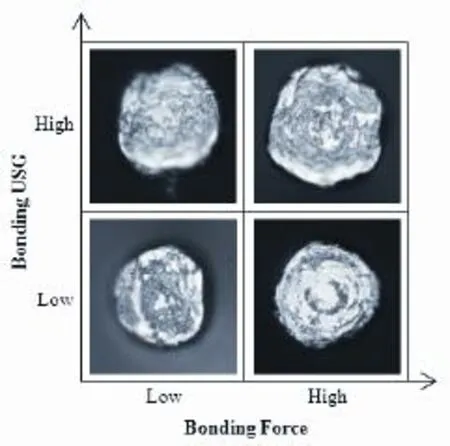
Fig. 29 IMC coverage of corner bonding conditions

Just as introduced above, the peak stresses at the bonding interface were just below the IC zone of capillary; in fact, the capillary dimensions did determine the stress distribution and had an important effect on the formation of final ball bond.

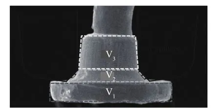
Fig. 30 Sketch of deformed ball bond

The deformed ball bond could be divided into 3 parts：squashed ball volume (V1), IC volume (V2) and neck back extrusion (V3), shown in figure-30. The ICA(inner chamfer angle) determined the IC volume and the final ball bond performance. Many experiments and simulations found that a smaller ICA got a bigger IC volume and a more even stress distribution in the deformed ball bond, just as shown in figure-31. This even stress distribution did help get a more stable performance of ball bond.

Un-optimized bonding parameters might result into a weak 1stbond which might lift off during wire bonding sometimes; and it was known as non-stick on pad (NSOP for short). This detection was implemented during the looping phase, so it would be introduced in the NSOP detection phase.

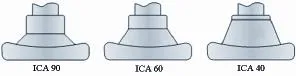
Fig. 31 Effect of ICA on IC volume

4 Phase III - Looping

4.1 Loop Reversing

After finishing the 1stbond, firstly the capillary ascended to a small height just above the 1stbond, which was called reversing height, shown in figure-32a. Then the capillary did a reversing kink and moved to the other location; the relative displacement between the end point and the beginning point of reversing motion (green point and purple point respectively in figure-32b) could be described with reversing distance and reversing angle,just as shown in figure-32b. Sometimes there might be more than one reversing motion for a more complex application of wire looping. Because the ascending was for the following reversing motion, they were combined together to be called the loop reversing phase here.

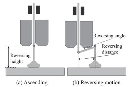
Fig. 32 Sketch of loop reversing phase

During the FAB forming phase, the wire tail melted into a liquid ball, and the immediate neighbouring region above the ball also reached to a high temperature due to the dissipation of heat and resulted into a recrystallized zone which was known as heat affected zone(HAZ for short). This HAZ had larger grains and lower strength, just as figure-33[13]showed, compared with the unaffected wire. The length of HAZ depended on the composition of bonding wire and EFO parameters mainly, and the typical HAZ length was within the range from 100 μm to 300 μm.

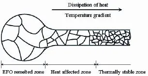
Fig. 33 Sketch of heat affected zone

Because the HAZ was softer, the wire loop was bended above it and the final loop height was higher than the HAZ to avoid damaging; just as showed in figure-34[14]. So the parameter of reversing height was recommended to be higher than the HAZ length of bonding wire.

Generally the part of wire loop just above the 1stbond was called ball neck. The speed of capillary ascending was called lifting speed and that of reversing motion was called kinking speed. Un-optimized reversing parameters (reversing height, reversing distance,reversing angle, lifting speed and kinking speed), poor or impeded wire path, and un-synchronal motion of XY-bond table and Z-axis all could affect the quality of ball neck. Figure-35 showed SEM images of good and damaged ball necks. The ball pull strength of a damaged ball neck after 500 temperature cycles was only 6.0 gf,while that of a good ball neck was above 12.0 gf.

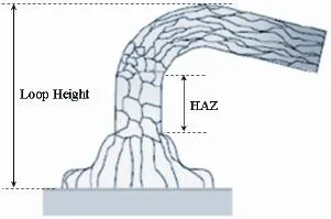
Fig. 34 Relationship between HAZ length and loop height

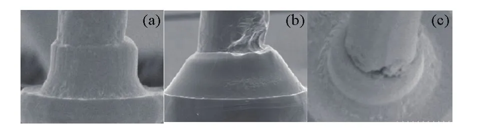
Fig. 35 SEM images of ball neck

4.2 Loop Ascending

After one or multi reversing motions, the capillary ascended to a peak height where the wire clamp was closed; then the wire wouldn’t be drawn out anymore and the NSOP (non-stick on pad) detection would be implemented. This ascending from the end of loop reversing to the peak height was called the looping ascending phase here, and the motion speed was called the ascending speed, shown in figure-36.

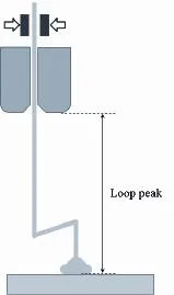
Fig. 36 Sketch of loop ascending phase

The peak height was called looping peak here and there are two paths of ascending to this peak location.As figure-37 showed, one was that the capillary moved vertically from point 1 to point 2 firstly, then horizontally from point 2 to point 3; the other was from point 1 to point 3 directly. The first path was used generally for a better looping stability. At the same time, there was an offset correction to the looping peak setting for a better loop profile output. A positive correction would lengthen the actual wire length and get a loose loop; while a negative correction would shorten the length and get a tight loop.

4.3 NSOP Detection

At the height of looping peak, the wire clamp was closed; and after waiting a time delay or a distance offset,the bonder started NSOP (non-stick on pad) detection which would end before the beginning of 2ndbond.

First of all, the basic electric circuit of NSOP detection would be illuminated as the example in figure-38 and these of other detections would be introduced respectively later. During the detection,the ball bond on the die was grounded and the EFO discharging box provided a voltage,V0, through the wire clamp; at the same time, the NSD board collected the voltage,V+, and compared it withV- through a voltage comparator. The comparison result depended on the circuit continuity or non-continuity which was determined by the bond quality. In the circuit, the electric resistance ofR1was bigger than that ofR2. For the NSOP detection, if the ball bond was stuck, the bond was grounded, the circuit was continuous,V+ was lower thanV- and the output was 0; and if the ball bond was nonstuck, the bond wasn’t grounded anymore, the circuit was non-continuous,V+ was higher thanV- and the output was 1. If the output was 1, there would be an alarm of NSOP.

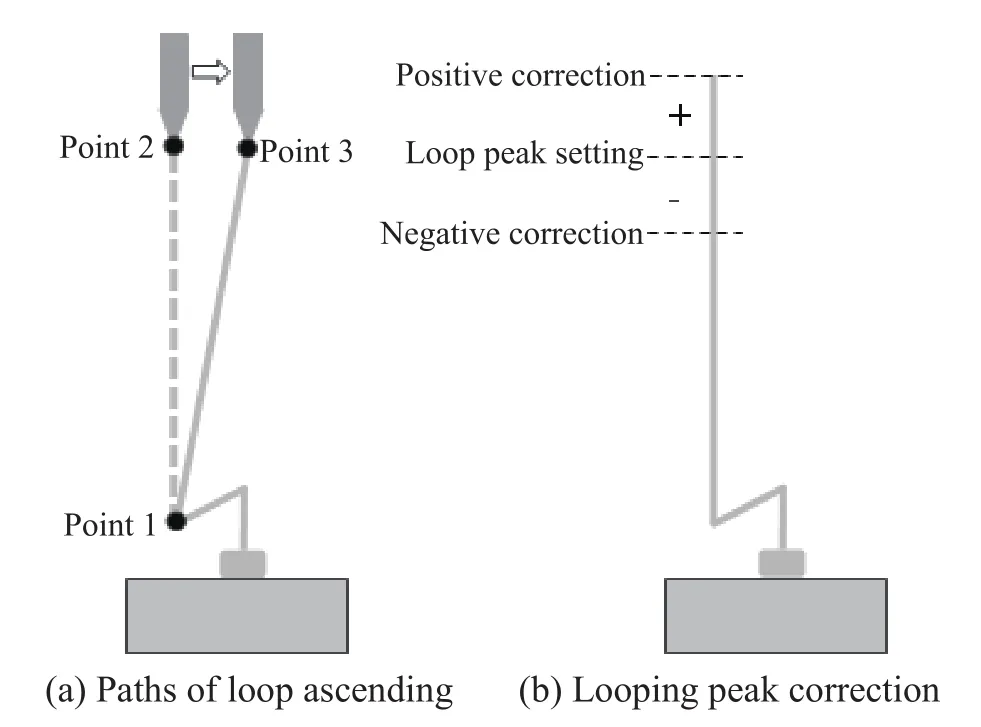
Fig. 37 Settings of looping peak

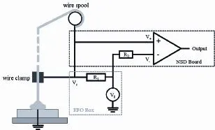
Fig. 38 Sketch of electric circuit for NSOP detection

In fact, there were two different kinds of detection method and relative setting. One was the comparison of continuity ratio. The detection lasting during the loop tracing phase which would be introduced later repeated some times, and one time was called a sample. Just as figure-39 showed, the 1stsample was the start point and the last one was the end point; and the typical sampling interval was 0.5 ms. For the NSOP detection, if the ratio of the continuity sample number to the total detection sample number was higher than a threshold, the bond would be considered as being stuck; or else being nonstuck. This threshold was called the NSOP sensitivity;a high setting would get more false alarms while a low setting would mask some true non-sticks. The other one was the comparison of voltage drop. The voltage drop between before and after closing the wire clamp would be compared with a threshold. If the actual drop was bigger, the bond was considered as being stuck; or else being non-stuck. Just as the NSOP sensitivity mentioned above, this threshold of voltage drop should be also set properly, and an improper setting would bring false alarms or mask true alarms.

Fig. 39 Sketch of detection sampling

About the electric circuit, there were two points which should be paid more attention on. The wire segment between the wire spool and the wire clamp wasn’t shielded by the wire bonder and might be touched easily; and this touching grounded this segment and masked true alarms of NSOP. Figure-40 showed this point.

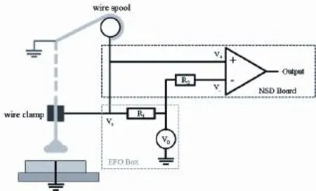
Fig. 40 Wrong grounding masking true NSOP

The other was shown in figure-41, the unconnection between the wire spool and the NSD board.From the analysis of electric circuit, this open might have little effect on the detection result; while this connection provided an additional circuit and enhanced the detection accuracy. In fact, there were many similar additional circuits in the wire bonder; the electric circuit in figure-38 was just a basic simplification.

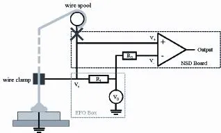
Fig. 41 Un-connection between wire spool and NSD board

4.4 Loop Tracing

From the looping peak to the beginning of 2ndbond,the capillary descended along a trajectory and it was called the loop tracing phase. The actual trajectory could be set according to the requirements of the final loop profile. Just as figure-42 showed, the trajectory 1 would get a loose loop while the trajectory 3 would get a tight loop finally. The motion speed was called the tracing speed.

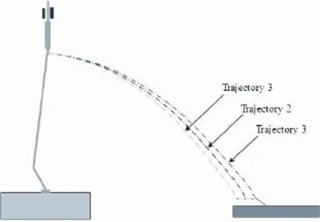
Fig. 42 Different trajectories for loop tracing phase

5 Phase IV - 2nd Bonding

5.1 Searching-2

At a height above 2ndbonding surface, the loop tracing phase ended and the searching-2 phase began.The height was called the searching height-2 where the wire clamp would be opened and the descending velocity would be decreased to a constant velocity, which was called the searching speed-2 (2 here meant 2ndbonding),shown in figure-43.

The parameters of searching speed-2 and searching height-2 were just like those of 1stbonding, while the approaching path to the 2ndbonding surface should be paid more attention on due to the existence of un-bonded loop.

There was a looping parameter, approaching angle,to determine the approaching path from the searching height-2 to the 2ndbond point. This parameter described the angle between the approaching path and the normal direction of 2ndbonding surface, shown in figure-44.If this angle was set as 0, the capillary would approach vertically. A higher setting of approaching angle helped to straighten the wire loop, while might introduce issues of short tail or weak 2ndbond. Figure-45 showed the images of loops changing approaching angle from 0 degree to 45 degree; the landing profile became straight while the stitch pull strength degraded about 1.5 gf averagely.

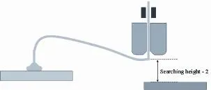
Fig. 43 Sketch of searching-2 phase

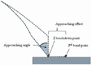
Fig. 44 Different approaching paths

Generally the Z touchdown point of capillary approaching was just the 2ndbond point. However, for some optimizations there was a parameter, approaching offset; which determined the relative dragging distance of capillary on 2ndbonding surface, by the motion of X-Y table of wire bonder. A dragging towards to 1stbond could increase the welding area of 2ndbond and reduced the peeling of tail bond; while a too long dragging might cause the wire dragging back or weak 2ndbond.

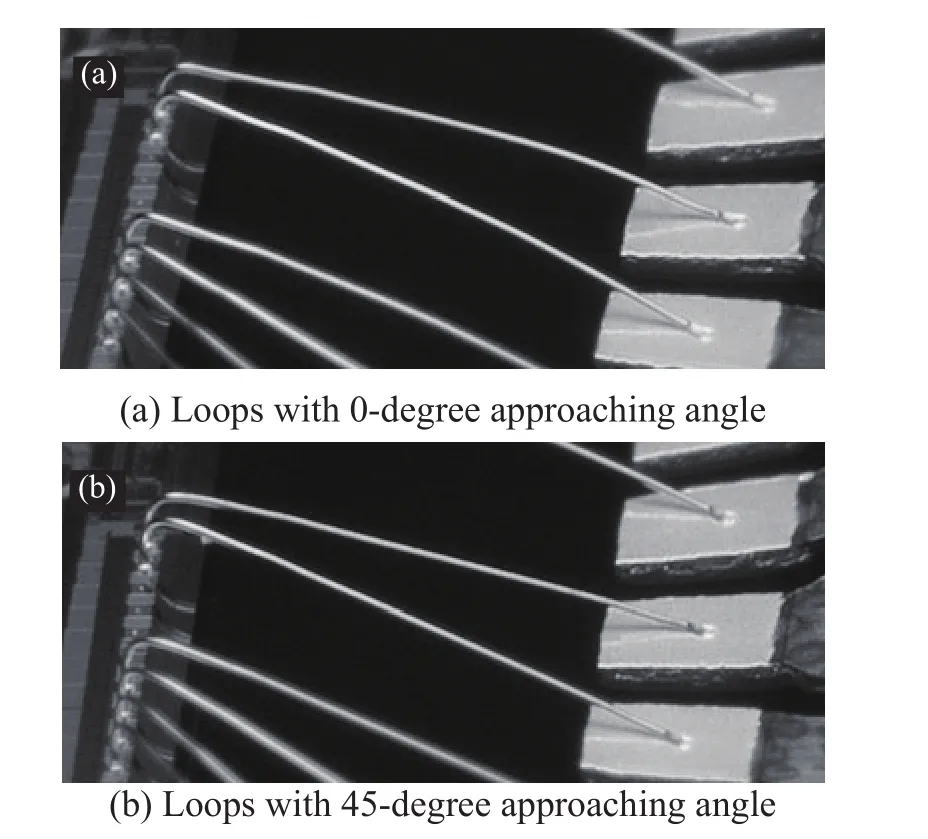
Fig. 45 Loops with different approaching angles

5.2 Impacting-2, Contacting-2 and Bonding-2

Just as the implementation of 1stbonding, after the searching phase the 2ndbonding also consisted of 3 phases：impacting, contacting as well as bonding; and the basic principles and main bonding parameters were similar. However, there were 2 points which should be emphasized additionally here.

The first one was the effect of bonding temperature on the quality of stitch bond. An experiment of effects of bonding temperature and post-bonding temperature on the stitch pull strength was implemented with 25.4 μm copper wire on a KNS maxum-plus wire bonder, and the 2ndbonding surface was silver-plated bare copper lead frame. The strength values were listed in figure-46 and the relationship was regressed into the equation-3 with statistic software. The bonding temperature had positive effect greatly; however, too high bonding temperature also might introduce unexpected issues, such as oxidation of bonding surface and package delamination.

Stitch pull strength=8.28+0.76×[(Bonding Temp-215)/15]-0.21×[(Bonding Temp-215)/15]×[(Postbonding Temp-75)/25](3)

The other one was the effect of capillary dimensions on the quality of stitch bond, which would be discussed in the NSOL phase.

After the 2ndbonding phase, the tail bond was also formed along with the 2ndbond, just as figure-47 showed.The formation of tail bond was complex and important to both 2ndbonding and subsequence cycle, it would be introduced detailed in the tail tearing phase.

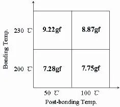
Fig. 46 Matrix of stitch pull strength values

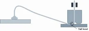
Fig. 47 Sketch of 2nd bond and tail bond

6 Phase V - Tailing

6.1 Tail Ascending

After finishing the 2ndbond, the capillary ascended a distance and left a wire tail for the subsequent bonding,shown in figure-48. The distance was commonly known as the tail length and the velocity of ascending was called the tailing speed. At the end of this tail ascending phase,the wire clamp would be closed for the following SHTL(short tail) detection.

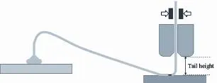
Fig. 48 Sketch of tail ascending phase

（未完待续）