A Double Iteration Process for Solving the Nonlinear Algebraic Equations,Especially for Ill-posed Nonlinear Algebraic Equations

Weichung YeihI-Yao ChanCheng-Yu KuChia-Ming Fan and Pai-Chen Guan

1 Introduction

The engineering or physical problems are sometimes modeled as nonlinear equations.After discretization,a system of nonlinear algebraic equations is then needed to be solved.Unlike the linear algebraic equation system,there exist not many solvers for the nonlinear algebraic equation system.Among these nonlinear equation solvers,they can be categorized into two folds:iteration and evolution dynamics.

For the group of iteration,most well-known methods are Newton’s method[T-jalling(1955)]and Landweber iteration method[Landweber(1951)].The former one is very efficient for solving nonlinear equation however it is not appropriate to adopt this method for the ill-posed system since the inverse of Jacobian matrix is not easy to obtain.The later one is less efficient than the Newton’s method while dealing with the well-posed problem but is more stable when dealing with the ill-posed problem.However,the Landweber iteration method cannot deal with severely ill-posed system and most of times the Tikhonov’s regularization method[Tikhonov and Arsenin(1977)]is required.

For the group of evolution dynamics,a system of the first order ordinary differential equations of the unknowns is constructed and the trajectory of the unknown will approach to the fixed point of this ODE system which is the solution of the original algebraic equation system[Ramm(2007)].The homotopy method[Billups(2002)],the scalar homotopy method[Liu,Yeih,Kuo and Atluri(2009)],the fictitious time integration method[Ku,Yeih,Liu and Chi(2009)]and so on can be categorized in this group.

No matter the iteration method or the evolution dynamic method is adopted,the unknown vector changes according to some known direction for most methods.For example,the Newton’s method uses the direction of B−1F where the superscript‘-1’denotes the inverse of a matrix,Landweber iteration method and the exponentially convergent scalar homotopy algorithm(ECSHA)[Chan,Fan and Yeih(2011)]use the direction of BTF.The fictitious time integration method(FTIM)and the dynamic Jacobian inverse free method(DJIFM)[Ku,Yeih and Liu(2011)]adoptthe direction of F.Liu[Liu and Atluri(2011a)]proposed to use two directions at the same time and he found the optimal combination of these two directions.[Yeih,Ku,Liu and Chan(2013)]extended this idea and answered the question for finding the optimal combination for multiple directions.All these methods adopt one or a combination of multiple known directions,however,generally speaking adopting a known direction or a combination of multiple known direction cannot guarantee it will be the best one for all problems.Later in the article,it will be found that theoretically the optimal direction will be the direction of B−1F if the inverse of the Jacobian matrix does exist.However,for the ill-posed problem or some special cases the inverse of the Jacobian matrix does not exist or cannot be found in the numerical sense the optimal searching direction used in the iteration process or evolution dynamics method is then not proposed to authors’best knowledge.To overcome the ill-posed nature,the abovementioned alternatives such as the Landweber iteration,the fictitious time integration method and so on adopt other directions than the direction of B−1F such that the numerical process will be stabler.The problem is these methods show slow convergence rate which makes solving the nonlinear ill-posed problem become not economic in numerical sense.Especially when the large scale problem is encountered,computation effort to deal with the ill-posed nature then becomes awful and not acceptable for engineers.

The method proposed here combine two recent developed methods:the residual norm based algorithm and the modified Tikhonov’s regularization method.The followings give a brief review of these two methods.Recently,the residual norm based algorithm(RNBA)has been proposed to deal with the nonlinear algebraic equation system.[Liu and Atluri(2012);Liu and Atluri(2011b)]The RNBA basically is a type of the scalar homotopy method[Liu,Yeih,Kuo and Atluri(2009)]where the trajectory of the unknown vector is required to lie on the space-time manifold.The RNBA constructs an iteration process from the evolution dynamics when the evolution direction u is selected.Later,Liu(2013)reported that the value of the relaxation parameter in RNBA has an optimal value.The modified Tikhonov’s regularization method(MTRM)[Liu(2012)]proposed an iteration to solve the solution for an ill-posed linear system.In the same paper,Liu also proposed a generalized Tikhnov’s regularization method(GTRM)to solve the ill-posed linear system.The MTRM is very similar to conventional Tikhonov’s regularization method which adds a regularization parameter in the diagonal line of the leading coefficient matrix while the GTRM adds regularization parameters in the diagonal line and the determination for these regularization parameters depend on the equilibrate matrix concept.

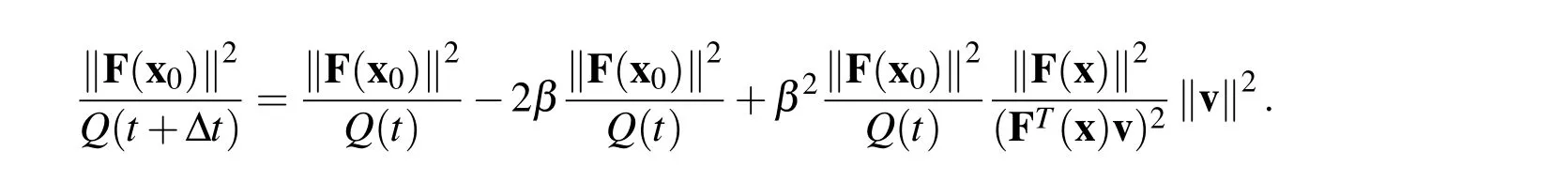
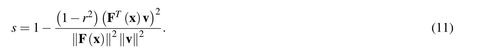
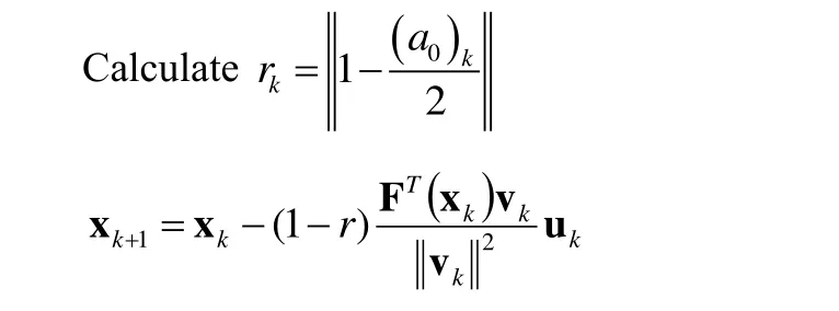
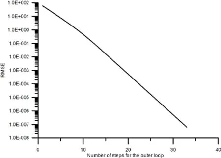
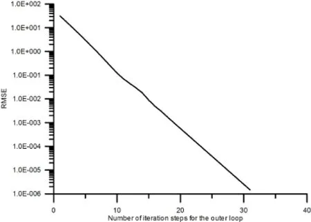
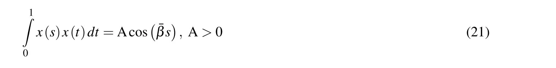
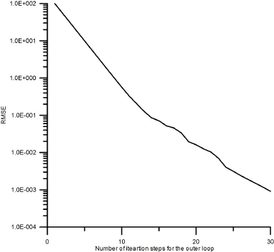
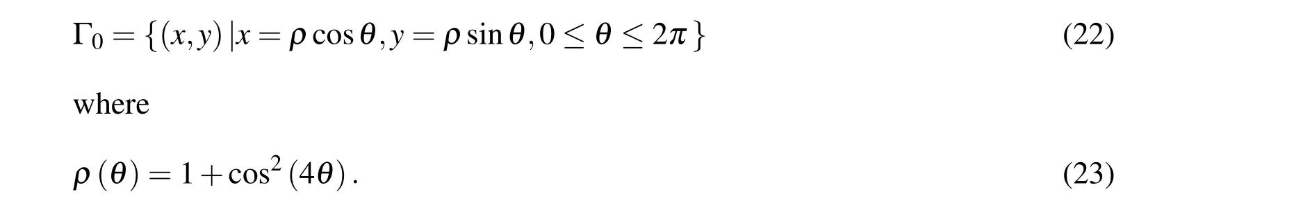
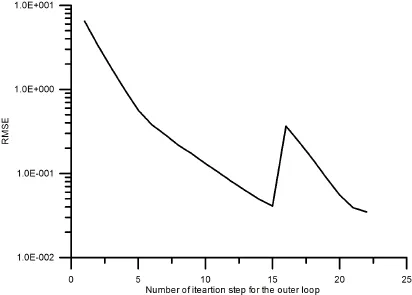
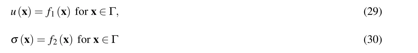
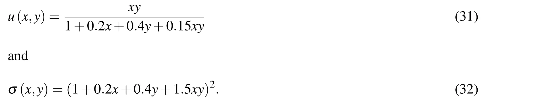
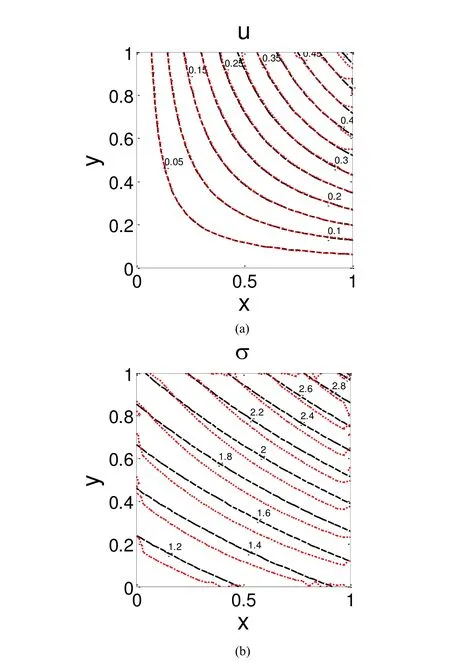
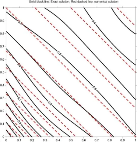
In this article,we develop a novel double iteration process to deal with the nonlinear algebraic equation systems.For outer iteration process,the evolution path of the unknown vector follows the searching direction determined from the inner iteration process and the process requires the path falls on the space-time manifold such that the convergence rate can be guaranteed.To determine the searching direction,we solve a linear algebraic equation system:BTBu=BTF.For a well-posed problem,it can be easily proved that the direction u for the above problem is B−1F.However,for the ill-posed problem the above linear system cannot be solved due to the ill-posed nature.We adopt the modified Tikhonov’s regularization method(MTRM)[Liu(2012)]to iteratively approach the solution for the above linear sys-tem.However,for ill-posed problems to really find the solution of u may require too many iteration steps for the modified Tikhonov’s regularization method which makes the whole numerical process not economic at all.Therefore,we propose that the inner iteration process should stop while the direction u already makes the value ofa0being smaller than the prescribed critical valueac(it should be smaller than 4 to guarantee the path falls on the manifold)or while the number of the iteration steps for the current inner iteration process exceeds the prescribed maximum tolerance value says Imax.The former criterion loosen the problem for solving BTBu=BTF exactly(for which the value ofa0should be one exactly)by finding an approximated direction such thata0

2 Mathematical backgrounds

2.1　Residual Norm Based Algorithm(RNBA)

The following derivation can be found in many related articles such as[Liu and Atluri(2012);Liu and Atluri(2011b)].Let us begin with a nonlinear algebraic system written as:

where F denotes the residual vector and x denotes the unknown vector.To solve this nonlinear algebraic equation system,we formulate an equivalent scalar equation written as

It is obvious that solving equation(1)is equivalent to solving equation(2)and vice versa.Now let us construct a space-time manifold as:

where x0is the initial guess andQ(t)satisfies thatQ(t)>0,Q(0)=1,and it is a monotonically increasing function oftwithQ(∞)=∞.

In order to keep the trajectory of the solution x on the manifold,the following consistency equation should be satisfied:

whereλis the proportional constant.After some manipulations,we can obtain the evolution equation of x as

where v=Bu.Now let us consider the evolution of the residual vector as:

Substituting equation(6)into equation(7),we then obtain:

Using the forward Euler scheme,we can discretize equation(8)as:

Consequently,an algebraic equation forβis obtained as:

Now let us use the forward Euler scheme on equation(6),we can obtain the following equation

For a selected value ofr,we can rewrite equation(12)as an iteration formula[Liu and Atluri(2011b)]:

In the above equation,the relaxation parameter is used to make the iteration stabler.In a recent published paper,Liu(2013)further found the value ofrneeds to satisfy the following relationship to guarantee the trajectory of x remains on the manifold:

3 Modified Tikhonov’s Regularization Method(MTRM)

The regularization technique is well-known for dealing with an ill-posed system.There exist many literatures mentioning the regularization technique.For readers’convenience,the following references can provide a conceptual understanding for the regularization technique.[Lin,Chen and Wang(2011);Wang,Chen and Ling(2012);Fu,Chen and Zhang(2012)]

The details of the following descriptions can be found in[Liu(2012)].Considering the following linear algebraic system as:

and we use the following preconditioner written as:

where B+is the pseudo-inverse with B+B=I.

and apply this preconditioner to equation(15)then we will obtain

It is quite interesting to find that the regularized equation in equation(17)is very similar to that of the conventional Tikhonv’s regularization method.However,in equation(17)the regularization parameter appears in the both sides of equation while for the conventional Tikhonov’s regularization method it appears only in the left-hand side.

Liu(2012)proposed that one can use equation(17)to formulate an iteration process as:

The convergence criterion of the iteration process for equation(18)can be set as:kup+1−upk≤ςwhereςis a preselected small tolerance.Liu also provided a theoretical proof of the convergence as the following theorem states:

[Theorem 1]For Eq.(18)with¯α>0 the iterative sequence upconverges to the true solution utruemonotonically.

Although the convergence of the sequence is guaranteed,in computation reality to reach the final numerical convergence it may takes too many steps such that it becomes not economic at all.It means that if one tries to find the solution of an ill-posed linear system,a lot of computation effort will be paid for the iteration process(equation(18))and sometimes it makes this iteration not economic at all.This algorithm needs to be further examine while it is used to solve the best direction u such that Bu-F=0 since for each step in the iteration process stated in equation(13)for solving the nonlinear problem this linear algebraic equation Bu-F=0 needs to be done if one tries to find the optimal direction.However,to find the solution of this linear problem may cost too many iteration steps for iteration process equation(18).Remember that we are not really interested in finding the best direction we only want to find an appropriate u such thata0is between 1 and 4.Therefore,we can check this criterion for each step of the inner iteration(equation(18))and terminate the inner iteration as the value ofa0is less than a prescribed critical valueac.Of course,it may take too many steps to leta0being less than this prescribed critical valueac.We say that if the number of iteration steps for the inner loop exceeds a preselected maximum number Imax,we then stop the inner loop as well as the outer loop.It means that to find an appropriate direction of evolution using the proposed algorithm already becomes not economic and the whole process should be terminated.

4 Double Iteration Process(DIP)

Based on the abovementioned theoretical backgrounds,we proposed a double iteration process as the followings.

Double Iteration Process(DIP):

Give initial guessx0

Outer Iteration:

Fork=0,1,2,… Repeat

Calculate the residual vectorFk(xk) and the Jacobian matrixBk(xk)

Inner Iteration:

(b) Ifp=Imax, terminates the whole process.

End of Inner Iteration

If RMSEe£ or (b) is true then the outer iteration process stops; otherwise continue.

End of Outer Iteration Process.

It is worth mentioned here that the initial guess in the inner iteration uses the descent direction.Actually,one can select other alternatives such asu0=0.How the initial guess for the inner iteration process influences the accuracy and efficiency of DIP leaves as an open question and in this article we use the initial guess as mentioned above.The DIP can be summarized in the flow chart in Fig.1.

Figure 1:The flow chart of DIP.

From the abovementioned double iteration process,we can find that the proposed method does not really try to solve the linear algebraic equationBu-F=0since it is expected that for the ill-posed system it may take too many iteration steps to accomplish this for the inner iteration and it definitely costs too much.In order to avoid using much computation effort,we say once the value ofa0is less than the prescribed valueacwe claim that the appropriate direction has been found already.Of course we need to remind ourselves that whileacapproaches to one the inner iteration takes more and more steps.And we expect that to find an appropriate direction may still require unreasonably many steps so we say that once the iteration steps exceed that maximum value Imaxwe can stop the whole process since it becomes not economic for further searching.The appropriate values ofac,¯αand Imaxinfluence the convergence speed a lot and how to choose them leaves as an open question.

According to our numerical experiences,the value ofacis suggested to in the range from 2.5 to 4.Once the value ofacis less than 2.5,to seek the appropriate direction in the inner loop then consumes too many iteration steps.The value ofimaxactually depends on the selection ofac.If the value ofacis between 2.5 and 4,the value ofimaxis suggested to be in the range of 30,000 to 80,000 according to our numerical experiences.The selection ofεdepends on the system we want to solve.If the system is a well-posed system,the value ofεcan be very small such as 10−7.However,if the system is an ill-posed system the value ofεshould not be very big and usually 10−3or 10−4is appropriate.It should be mentioned here that actually for an ill-posed system the value ofεcan be set as a small value for DIP since this tight convergence criterion cannot be reached and the whole DIP will be terminated due to the number of the inner iteration steps exceeds the maximum value Imax.It means the selection ofεis not critical at all.The value of¯αneeds to be larger than the smallest eigenvalue of BTB which varies step by step.In calculation reality,a big enough value is selected.However,if¯αis too big the iteration process for eq.(18)becomes slow.

5 Numerical Examples

[Example1]In this example,we consider an almost linear problem[Brown(1973)]:

Figure 2:The RMSE versus the number of steps for the outer loop in example 1.

Figure 3:The value of a0never exceeds ac.

[Example 2]In this problem,we consider the following simple system:

Figure 4:The absolute error for the k-th component in the solution vector x.

Figure 5:Trajectory for the solution using the Newton method.

Figure 6:RMSE versus the number of iteration steps for the outer loop in example 2.

Figure 7:The value of a0 never exceeds the critical value ac=2.0.

Figure 8:The trajectory of the solution for the double iteration method.

This is an interesting example because the iteration for Newton’s method fails when the initial guess is selected as(3,5)as shown in Fig.5.As the trajectory approaches tox1=3.5192 during the iteration,it happensx2≈0.0.It then is found that the Jacobian matrix now is nearly singular.This leads the trajectory of(x1,x2)oscillates at the axis forx1=3.5192 as shown in Fig.5.It means that the conventional Newton method fails for this case.We now use the double iteration process to solve this problem with the initial guess is set as(x1,x2)=(3,5).The parameters used for the double iteration process are¯α=10,ac=2.0,Imax=30000 andε=10−6.It is found from Fig.6 that the process terminates after 31 steps for the outer loop.We check the plot ofa0as shown in Fig.7 and we find out thata0never exceeds the critical valueac=2.0 which once more shows that our method really can guarantee the trajectory of the solution vector falls on the manifold.The trajectory of the solution is shown in Fig.8.

[Example 3]A classical example of an ill-posed problem is the nonlinear Fredholm integral equation of the first kind which is well known as a nonlinear ill-posed problem.The problem we consider is written as:

where A and¯βare constants.We let A=1 and¯β=3 in the followings.We give data for Acos(¯βs)in the regions∈[0,1]by equally dividing the region into 200 segments,that means totally 201 data points are used.The data has disturbed by maximum 5%relative error.Therefore,we also use these 201 points as the integration quadrature points and the trapezoidal rule is used for integration.

and Manzhirov(2007)].The initial guess are given asx(t)=10.0 fort∈[0,1]and the following parameters are used:¯α=0.1,ac=2.5,Imax=30000 andε=10−3.The reason why the value ofεis not very small in comparison with the previous two examples is that this problem is ill-posed in nature and therefore the convergence criterion can be larger.From Fig.9,one can find that after 30 steps for the outer loop the solution converges to the requirement.It can be found from Fig.10 that the numerical solution is acceptable for an ill-posed problem with maximum 5%relative absolute random error in data.The relative absolute random error percentage(RAREP)for a given dataxgiven(from numerical calculation or prescribed value)is defined as:

The proposed method shows excellent noise resistance for the ill-posed nonlinear problem.

[Example 4]The following problem appeared in[Chan and Fan(2013)].Here we consider a boundary detection problem with the governing equation is the biharmonic equation.The boundary enclosing the computational domain is defined by

Figure 9:RMSE versus number of iteration steps for the outer loop in example 3.

Figure 10:The solution of a Fredholm integral equation of the first kind.

the parametric equation:

For 0≤θ≤π,we prescribe four boundary data as

Forπ<θ≤2π,only the Dirichlet boundary data is given but the geometry or the lower part is missing.We assume that the designed field property is written as:

To recover the missing boundary and solve the field quantity at the same time makes this problem becomes a nonlinear ill-posed inverse problem.To solve this problem,we adopt the same discretization method used in[Chan and Fan(2013)],that means the modified Trefftz collocation method is used.Forthe known boundary,totally 60 points are arranged and 40 points are used for the unknown boundary and the initial guess of the missing boundary is a half circle.The characteristic length used in this problem is 3.0 and the order for the basis is 24.That means totally we have 98 Trefftz basis functions,for more details please refer to[Chan and Fan(2013)].The parameters used for double iteration process are:¯α=10,ac=2.5,Imax=50000 andε=10−3.It can be found from Fig.11 that the RMSE never reaches the requirement and the whole process terminates for the number of iteration steps for the inner loop is equal to 22.The reported CPU time is 106.69 sec using the Pentium®dual core CPU E5200 at 2.5GHz.The accumulated steps for the inner loop are 70659 steps.We further examine the plot ofa0as shown in Fig.12,the value ofa0exceeds the critical valueacand it seems that further seeking an appropriate vector u becomes numerically uneconomic.However,we can find in Fig.13 that the recovering shape for the missing boundary is already acceptable.The proposed method can automatically stop while further reducing the norm of residual vector becomes difficult and stops at that time still yield acceptable result.

Figure 11:RMSE versus the number of iteration step for the outer loop in example 4.

Figure 12:The value of a0 exceeds ac in example 4.

Figure 13:The recovery of missing boundary.(-.-:known boundary;-.-:initial guess for the unknown boundary;-+-:exact unknown boundary;-+-:recovery of missing boundary using data with maximum 1%relative error)

[Example 5]In the following,an inverse problem is given as:

where Ω is the interested domain.

The field quantityuand the conductivityσis both unknown.The boundary values of the field quantity and conductivity are given as boundary conditions:

where Γ is the boundary enclosed the interested domain.The domain we consider is a square region andx∈[0,1]andy∈[0,1].The designed exact solutions for the field quantity and the conductivity are given as

We use finite difference to discretize the domain by using a 31 by 31 mesh.Maximum 5%relative random errors are added in the data both in the surface field quantity as well as the surface conductivity.The parameters used for the double iteration process are:¯α=0.1,ac=2.5,Imax=30000 andε=10−5.It reports that the process terminates for the number of steps for the outer loop is equal to 22 and the RMSE is lower than the requirement.The solutions for the field quantity and the conductivity are shown in Fig.14(a)and(b),respectively.The absolute error of the field quantity is illustrated in Fig.15(a)while the relative error of the conductivity is illustrated in Fig.15(b).The absolute error(AE)is de fined as:

whereunumis the numerical solution andutrueis the analytic solution.

From these figures,we can say that the current approach gives accurate result and this method has good noise resistance.

[Example 6]In the following,a nonlinear inverse Cauchy problem for a quasi-linear PDE is considered as:

in a square region withx∈[0,1]andy∈[0,1].

The Cauchy boundary conditions are given onx=0 andx=1 while no boundary data are given ony=0 andy=1.Maximum 2%relative random errors are added into 30×30 mesh for the domain and boundary.It means we have 120 boundary points and 780 inner points.Parameters used for the double iteration process are:¯α=0.01,ac=3.5,Imax=50000 andε=10−4.The initial guess for the weight of each radial basis function is equal to 0.001.After we obtain the weights for each radial basis functions,we use total 60x60 mesh to represent the solution.The contours for the exact solution and numerical solution are given in Fig.16.Although this result is not so well as previous examples,for an ill-posed nonlinear system like this problem it is acceptable.The relative error percentage contour plot is illustrated in Fig.17 and one can see that the maximum relative error percentage is about 5%while the maximum error in the boundary data is 2%which indicates that nonlinearity of the system may amplify the error.It should be mentioned here that in this case the process is terminated because the number of steps of inner loop exceeds Imax=50000.

Figure 14:Numerical solutions for(a)the field quantity(b)the conductivity.(-+-:the exact solution;—:numerical solution)

Figure 15:Error distribution:(a)absolute error for the field quantity;(b)absolute relative error for the conductivity.

Figure 16:Comparison between the exact solution and the numerical solution.

Figure 17:The absolute relative error percentage contour plot for example 6.

6 Conclusions

In this paper,a novel double iteration process for solving the nonlinear ill-posed system is proposed.The appropriate direction of evolution is determined from the inner loop which is based on the modified Tikhonov’s regularization method.In order to avoid consuming too much computation effort,the whole process will be terminated when the number of iteration steps for the inner loop exceeds the maximum prescribed value.In such a case,it is said to further seek for the appropriate direction of evolution is computationally uneconomic and thus one should stop whole process.However,from numerical results we can observe that the numerical result is still acceptable.In other words,the proposed method is efficient and robust for solving the nonlinear ill-posed systems.Six examples are given to illustrate the validity for the proposed method.

Acknowledgement:The authors would like to express their thanks to H.F.Chan and C.L.Kuo for providing information and related source codes for our modification in example 4 and example 5.

Billups,S.C.(2002):A homotopy-based algorithm for mixed complementarity problems.SIAM J.Optim.,vol.12 pp.583-605.

Brown,K.M.(1973):Computer oriented algorithms for solving systems of simultaneous nonlinear algebraic equations.In Numerical Solution of Systems of Nonlinear Algebraic Equations,Byrne,G.D.and Hall C.A.Eds.,pp.281-348,Academic Press,New York.

Chan,H.F.;Fan,C.M.(2013):The modified collocation Trefftz method and exponentially convergent scalar homotopy algorithm for the inverse boundary determination problem for the biharmonic equation.Journal of Mechanics,vol.29,pp.363-372.

Chan,H.F.;Fan,C.M.;Yeih,W.(2011):Solution of inverse boundary optimization problem by Trefftz method and exponentially convergent scalar homotopy algorithm.CMC:Computers,Materials,&Continua,vol.24,pp.125-142.

Fu,Z.J.;Chen,W.;Zhang,C.Z.(2012):Boundary particle method for Cauchy inhomogeneous potential problems.Inverse Problems in Science and Engineering,vol.20,no.2,pp.189-207.

Ku,C-Y;Yeih,W(2012):Dynamical Newton-like methods with adaptive stepsize for solving nonlinear algebraic equations.CMC:Computers,Materials,&Continua,vol.31,pp.173-200.

Ku,C-Y;Yeih,W;Liu,C-S(2011):Dynamical Newton-like methods for solving ill-conditioned systems of nonlinear equations with applications to boundary value problems.CMES:Computer Modeling in Engineering&Sciences,vol.76,pp.83-108.

Ku,C.-Y.;Yeih,W.;Liu,C.-S;Chi,C.C.(2009):Applications of the fictitious time integration method using a new time-like function.CMES:Computer Modeling in Engineering&Sciences,vol.43,pp.173-190.

Landweber,L.(1951):An iteration formula for Fredholm integral equations of the first kind.Amer.J.Math.,vol.73,pp.615–624.

Lin,J.;Chen,W.;Wang,F.(2011):A new investigation into regularization techniques for the method of fundamental solutions.Mathematics and Computer in Simulation,vol.81,no.6,pp.1144-1152.

Liu,C.-S.(2008):A fictitious time integration method for two-dimensional quasilinear elliptic boundary value problems.CMES:Computer Modeling in Engineering&Sciences,vol.33,pp.179-198.

Liu,C.-S.(2012):Optimally generalized regularization methods for solving linear inverse problems.CMC:Computers,Materials,&Continua,vol.29,pp.103-127.

Liu,C.-S.(2013):An optimal preconditioner with an alternate relaxation parameter used to solve ill-posed linear problems.CMES:Computer Modeling in Engineering&Sciences,vol.92,pp.241-269.

Liu,C.S.;Atluri,S.N.(2011a):An iterative algorithm for solving a system of nonlinear algebraic equations,F(x)=0,using the system of ODEs with an optimum in˙x=λ?αF+(1−α)BTF?;Bij=∂Fi/∂xj.CMES:Computer Modeling in Engineering&Sciences,vol.73,pp.395431.

Liu,C.-S.;Atluri,S.N.(2011b):Simple"residual-norm"based algorithms,for the solution of a large system of non-linear algebraic equations,which converge faster than the Newton’s method.CMES:Computer Modeling in Engineering&Sciences,vol.71,pp.279-304.

Liu,C.-S.;Atluri,S.N.(2012):An iterative method using an optimal descent vector,for solving an ill-conditioned system BX=b,better and faster than the conjugate gradient method.CMES:Computer Modeling in Engineering&Sciences,vol.80,pp.275-298.

Liu,C.-S.;Yeih,W.;Kuo,C.L;Atluri,S N.(2009):A scalar homotopy method for solving an over/under-determined system of non-linear algebraic equations.CMES:Computer Modeling in Engineering&Science,vol.53,pp.47-71.

Polyanin,A.D.;Manzhirov,A.V.(2007):Handbook of Integral Equations.Second Edition,Caoman&Hall/CRC,Taylor&Francis Group,New York.

Ramm,A.G.(2007):Dynamical system methods for solving operator equations.Mathematics in Science and Engineering,vol.208 Elsevier,Amsterdam,Netherlands.

Tikhonov,A.N.;Arsenin,V.Y.(1977):Solution of Ill-posed Problems.Washington:Winston&Sons.

Tjalling,J.Y.(1955):Historical development of the Newton-Raphson method.SIAM Review,vol.37,pp.531–551.

Wang,F.;Chen,W.;Ling,L.(2012):Combinations of the method of fundamental solutions for general inverse source identification problems.Applied Mathematics and Computation,vol.19,no.3,pp.1173-1182.

Yeih,W.;Ku,C-Y;Liu,C.-S;Chan,I-Y(2013):A scalar homotopy method with optimal hybrid search directions for solving nonlinear algebraic equations.CMES:Computer Modeling in Engineering&Sciences,vol.90 pp.255-282.