Lattice Boltzmann Flux Solver：An Efficient Approach for Numerical Simulation of Fluid Flows＊

Shu Chang，Wang Y，Yang L M，Wu J

1.Department of Mechanical Engineering，National University of Singapore，10Kent Ridge Crescent，Singapore，119260；2.College of Aerospace Engineering，Nanjing University of Aeronautics and Astronautics，Nanjing，210016，P.R.China（Received 20January 2014；revisied 18February 2014；accepted 22February 2014）

1 Introduction

Computational fluid dynamics（CFD）is to apply a numerical method to solve governing equations of fluid flows on the computer.Among various numerical methods available［1－8］，the finite volume method（FVM）is the most popular approach in CFD.This is because numerical discretization by FVM is in line with application of physical conservation laws to a control cell.The discrete forms of governing equations by FVM usually involve the conservative variables at cell centers and numerical fluxes at cell interfaces.From numerical point of view，only the conservative variables at cell centers are defined as unknowns，which can be given from the solution of discrete governing equations.In the solution process，we need to use conservative variables at cell centers to evaluate numerical fluxes at cell interfaces.This process is often termed flux solver.Currently，there are three major flux solvers in CFD.One is based on the smooth function approximation.In this solver，a smooth function，which could be a polynomial［9］or a radial basis function［10］，is applied to approximate the solution in the local region.The coefficients in the smooth function can be determined by collocation method.Once the smooth function is decided，its integral or derivative can be given in a straightforward way.It should be noted that this solver is a mathematical approach，which can be applied to general engineering problems.However，this solver cannot resolve discontinuity problems such as compressible flows with shock wave.To re－solve shock wave problems in CFD，the Riemann solver or approximate Riemann solver is often used.The pioneer work in this category was made by Godunov［11］，who simplified the compressible flow into a series of Riemann problems and then solved one－dimensional（1D）Euler equations to get local solution.After the work of Godunov［11］，various approximate Riemann solvers were presented［12－16］.These solvers usually pursue approximate solution of 1DEuler equations along the normal direction to the cell interface.Thus，they can only be used to evaluate inviscid flux.For compressible viscous flows，the viscous flux is still evaluated by the smooth function approximation.In the literature，there is another type of flux solver called gas kinetic flux solver［17－19］，which evaluates inviscid and viscous fluxes simultaneously from local solution of multi－dimensional Boltzmann equation.The solvers in this category can be well applied to simulate both incompressible and compressible flows.But they are usually more complicated and less efficient than the smooth function－based solvers and Riemann solvers.In this paper，we will present a new flux solver，which is based on local solution of lattice Boltzmann equation（LBE）.

In recent years，lattice Boltzmann method（LBM）［20－32］has received more and more attention due to its simplicity，easy implementation and parallel nature.In LBM，the density distribution functions are taken as unknowns and LBE is an algebraic formulation.Once the density distribution functions are known at a physical location，the macroscopic flow variables such as density and velocity can be easily computed from local conservation laws of mass and momentum.No differential equation and solution of algebraic equations are involved in the LBE solver.On the other hand，it is indicated that LBE solvers also suffer from some drawbacks.Due to uniformity of the lattice，the standard LBE solver is limited to the simple geometry and uniform mesh.For complex geometry and application on the non－uniform mesh，additional efforts such as interpolation have to be incorporated.The process may in－crease the complexity of the solver，and requires additional computational effort and virtual storage.The second drawback is the tie－up of time interval with mesh spacing.This drawback makes the adaptive and multi－block computation of LBE solvers extremely complicated.In addition，LBE solvers need more memory to store density distribution functions than the Navier－Stokes（N－S）solvers.Another drawback is that LBE solvers can only be applied to simulate viscous flows.Furthermore，the physical boundary conditions such as given pressure cannot be implemented directly in the LBE solver.As will be shown in this paper，all the above drawbacks of LBE solvers are completely removed by the lattice Boltzmann flux solver（LBFS）.

LBFS is based on Chapman－Enskog（C－E）expansion analysis，which is a bridge to link N－S equations and LBE.Usually，the C－E analysis is applied in the whole flow domain to verify that the macroscopic flow variables obtained by LBE solvers at any physical location and any time level can satisfy N－S equations.On the other hand，it was found that the C－E analysis can be applied at any location within a small streaming step.This idea has been well applied by Xu［17］in the development of gas kinetic scheme，where the flux at the cell interface is computed by local solution of BGK equation.In this work，the numerical fluxes at the cell interface are evaluated by local reconstruction of LBE solution.Two versions of LBFS are presented in this work.One is to locally apply 1Dcompressible LB model along the normal direction of cell interface for evaluation of inviscid flux.This version is only applicable for simulation of compressible inviscid flows.The other is to locally apply multi－dimensional LB model at the cell interface for evaluation of viscous and inviscid fluxes simultaneously.The performance of present LBFS will be investigated through some test examples.Numerical results demonstrate that LBFS can accurately and effectively simulate fluid flows with curved boundary and non－uniform mesh.It also removes the drawbacks of conventional LBM.

2 Lattice Boltzmann Flux Solver（LBFS）for Compressible Inviscid Flows

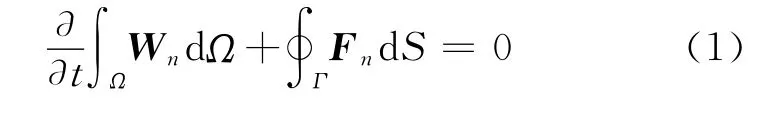
The integral form of Euler equations without source term can be written as

where the conservative flow variables Wand inviscid flux Fnare given by

whereρand pare the density and pressure of the mean flow，respectively.U＝（u，v，w）is the velocity vector in the Cartesian coordinate system and n＝（nx，ny，nz）denotes the unit normal vector on the control surface.Unrepresents the normal velocity，which is defined as the scalar product of the velocity vector and the unit normal vector，i.e.

Eis the total energy of the mean flow，which is defined as

Here e＝p／［（γ－1）ρ］is the potential energy of the mean flow，andγis the specific heat ratio.On the control surface，the tangential velocity Uτ＝ （Uτx，Uτy，Uτz）can be computed by

Applying Eq.（1）to a control volume gives

where Iis the index of a control volume，ΩIand Nfrepresent the volume and the number of the faces of the control volume I.dSidenotes the area of the ith face of the control volume.As indicated in the introduction，the flux solver needs to reconstruct numerical flux Fnat each cell interface from the conservative variables WIat cell centers.In this section，Fnwill be computed from the solution of 1Dcompressible LB model to a local Riemann problem.When 1DLB model is applied along the normal direction to the cell interface，only density，pressure and normal velocity are involved.Thus，before we address how to apply the 1Dcompressible LB model to reconstruct Fn，it is better to rewrite expression of Fnin terms of density，pressure，normal velocity and tangential velocity.From Eq.（5），we can express the velocity components in the Cartesian coordinate system in terms of normal velocity and tangential velocity as

Using Eq.（7）and the expression of potential energy，Fncan be rewritten as

It can be seen clearly from Eq.（8）that，to evaluate numerical flux Fn，we need to know the density，pressure，normal velocity and tangential velocity at the cell interface.This task can be fulfilled by local application of 1Dcompressible LB model to the Riemann problem defined at cell interface.In this work，the non－free parameter D1Q4LB model presented in Refs.［33－34］is adopted.This model is derived from conservation forms of moments，which can be used to simulate hypersonic flows with strong shock waves.The non－free parameter D1Q4model is shown in Fig.1.The equilibrium distribution functions and lattice velocities of this model are given below，where giis the equilibrium distribution function in the ith direction of phase space，diis the lattice velocity in the ith direction，c is the peculiar ve－locity of particles defined as c＝（Dis the dimension of space）.Note that when the above 1Dmodel is applied along the normal direction to the cell interface，u has to be replaced by Un.

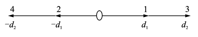
Fig.1 Configuration of non－free parameter D1Q4model

Next，we will show how to apply the nonfree parameter D1Q4model to evaluate Fnat cell interface.As shown in Fig.1，at any physical location，D1Q4model has 4moving particles.Now，we consider a local Riemann problem around a cell interface as shown in Fig.2.To compute Fn，we need to know distribution functions of 4moving particles at the cell interface.In the framework of LBM，the moving particles are actually streamed from neighbouring points.As illustrated in Fig.3，by giving a streaming step δt，particles 1and 3from left side of interface will stream to the cell interface while particles 2and 4 from right side of interface will also stream to the cell interface.Mathematically，the streaming process provides the distribution functions of four moving particles at cell interface as

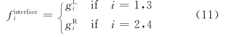
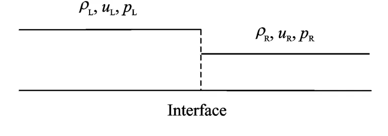
Fig.2 Configuration of a Riemann problem

Fig.3 Streaming process of D1Q4model at the cell interface

where gLiand gRiare the equilibrium distribution functions at the left and right sides of cell interface.For the Riemann problem，they are given from information at left and right cell centers.With flow variables，they can be computed by using Eq.（9）.With Eq.（11），there are two basic ways to evaluate the numerical flux Fnat the cell interface.The first way is to compute the flow variables（density，pressure and normal velocity）first，and then substitute them into Eq.（8）to compute Fn.The density，normal velocity and pressure can be computed by

where eiis the lattice velocity，e1＝d1，e2＝－d1，e is the po－tential energy of particles（Dis the dimension of space and takes 1for the 1Dmodel）.The tangential density Uτat the cell interface can be given from mean value of ULτand URτ，where ULτand URτare the tangential velocity at the left and right side of cell interface，respectively.Alternatively，it can be approximated by

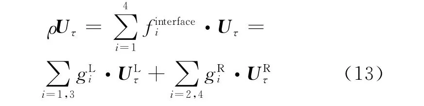
Once the density，pressure，normal velocity and tangential velocity at the cell interface are computed by Eqs.（12－13），they can be substituted into Eq.（8）to compute Fn.This way is equivalent to use equilibrium distribution functions at the cell interface to compute Fn.From CE analysis，this way has very little numerical dissipation，which may not be able to get stable solution for problems with strong shock waves.To compute Fnwith numerical dissipation，we can use distribution function given in Eq.（11）to compute Fndirectly.In fact，ρUnin Fnhas been calculated by Eq.（12b）.Other terms in Fncan be computed by the following formulations

Similar to Eq.（13），ρUnUτandρUn｜Uτ｜2can be approximated by

Overall，the basic solution procedure of this LBFS can be summarized below：

（1）At first，we need to choose a 1DLB model such as non－free parameter D1Q4model.The LB model provides expressions for equilibrium distribution functions and lattice velocities.

（2）For the considered cell interface with unit normal vector n＝ （nx，ny，nz），obtain flow variables（density，pressure，velocity components）at the left and right sides of interface from two neighbouring cell centers（MUSCL interpolation with limiter may be used for high－order schemes）.Then use Eqs.（3，5）to calculate the normal and tangential velocities at the left and right sides of interface.

（3）Use Eq.（9）to calculate gL1，gL3，gR2，gR4by using density，pressure and normal velocity.

（4）Compute the density，normal velocity，pressure and tangential velocity at the cell interface by using Eqs.（12－13），and then substitute them into Eq.（8）to calculate numerical flux Fn.Alternatively，use Eqs.（12b，14－17）to compute Fndirectly（this way is recommended for hypersonic flows with strong shock waves）.

（5）Once numerical fluxes at all cell interfaces are obtained，solve ordinary differential equations（6）by using 4－stage Runge－Kutta scheme.

For simulation of viscous flows，one also needs to use a smooth function to approximate the viscous flux.

3 Lattice Boltzmann Flux Solver（LBFS）for Incompressible Flows

From C－E expansion analysis［22，32］，the incompressible Navier－Stokes（N－S）equations

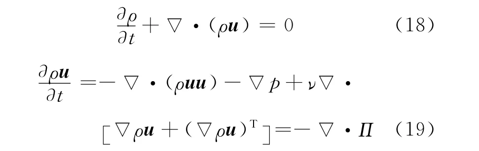
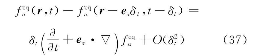
can be recovered by the following LBE

whereρis the fluid density，u the flow velocity and pthe pressure.r represents a physical location，τis the single relaxation parameter；fαis the density distribution function along theαdirection；feqαis its corresponding equilibrium state；δtis the streaming time step and eαis the particle velocity in theαdirection；Nis the number of discrete particle velocities.The relationships between the density distribution functions and flow variables as well as fluxes in the N－S equations are

whereβandγrepresent the space coordinate directions，and eαβis the component of the lattice velocity vector eαin theβ－coordinate direction.As shown in Refs.［22，32］，to recover N－S equations by Eq.（20），εf（1）αcan be approximated by

Substituting Eq.（24）into Eq.（23）gives

The equilibrium distribution functiondepends on the lattice velocity model used.For example，when the following two－dimensional D2Q9lattice velocity model

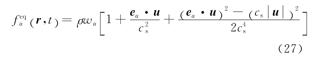
where c＝δx／δt，δxis the lattice spacing.For the case ofδx＝δt，which is often used in the literature and also adopted in this work，c is taken as 1.The coefficients wαand the sound speed csare given as：w0＝4／，w1＝w2＝w3＝w4＝1／9and w5＝w6＝w7＝w8＝1／36.cs＝.The relaxa－tion parameterτis linked to the kinematic viscosity of fluid through C－E expansion analysis by the following relationship

The pressure can be calculated from the equation of state by

Using Eqs.（22）and（23），for the two－dimensional case，Eqs.（18）and（19）can be rewritten as

where

When a cell－centered FVM is applied to solve Eq.（30），the flow propertiesρandρu at the cell center can be obtained by marching in time.The fluxes at the cell interface can be evaluated by local reconstruction of LBM solution.By integrating Eq.（30）over a control volumeΩi，we have

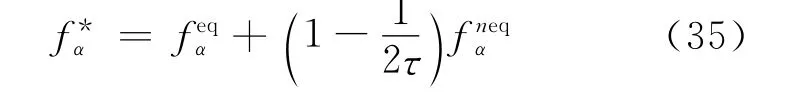
whereΔViis the volume ofΩi，andΔSkis the area of the kth control surface enclosingΩi.nxand nyare the xand ycomponents of the unit outward normal vector on the kth control surface.Obviously，once the fluxes at all cell interfaces are known，Eq.（34）can be solved by well established numerical schemes such as the 4－stage Runge－Kutta method.Thus，the evaluation of flux Rkat the cell interface is the key in the solution process.The detailed expression of Rkdepends on the lattice velocity model.By defining fas

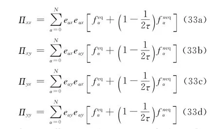
When the D2Q9lattice velocity model is used，Rkcan be written in detail as follows

Obviously，the key issue in the evaluation of the flux Rkis to perform an accurate evaluation of fandat the cell interface.In the following，we will show the detailed calculation ofand fat the cell interface.

Consider a cell interface between two control cellsΩiandΩi＋1as shown in Fig.4.It is assumed that the physical location for the two cell centers and their interface is ri，ri＋1and r respectively.

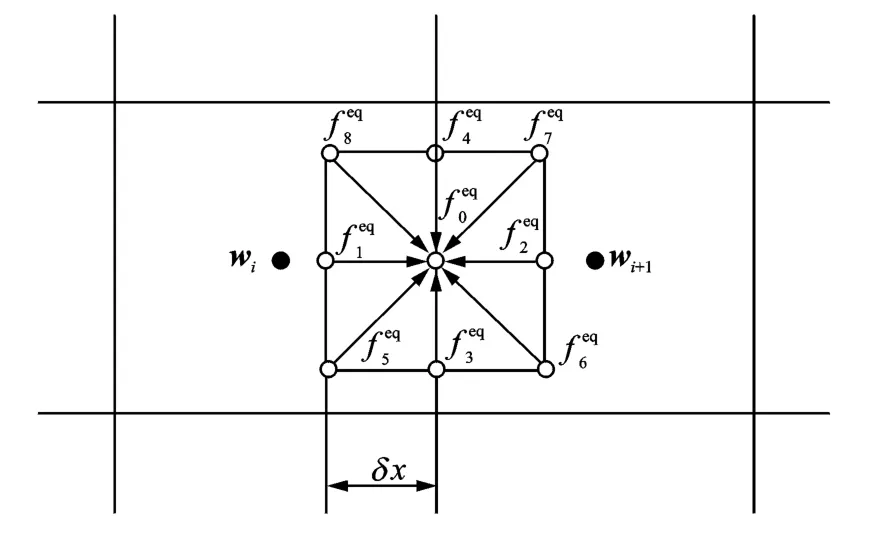
Fig.4 Local reconstruction of LBM solution at a cell interface

Using Taylor series expansion，we have

From Eqs.（37）and（24），we can get the following form

Eq.（38）shows that once we have the equilibrium distribution functions（r，t），（r－eαδt，t－δt）at the cell interface and its surrounding points，we can have the full information of distribution function at the interface.Note that the approximation for Eq.（38）is the second order of accuracy inδt.Using Eq.（27），the equilibrium distribution function feqαcan be computed from the fluid densityρand flow velocity u.With the given density and velocity at the cell center，the respective density and velocity at location（r－eαδt）can be easily obtained by interpolation.One of interpolation forms can be written as

With computedρ（r－eαδt）and u（r－eαδt）by Eqs.（39，40），（r－eαδt，t－δt）can be calculated by Eq.（27）.Now，we are only left to determine（r，t）as shown in Eq.（38）.Again，with Eq.（27），the calculation of（r，t）is equivalent to computingρ（r，t）and u（r，t）.Using Eqs.（21，22），the conservative variablesρandρu can be computed by

Since fαcan be written as，application of Eq.（20）at the cell interface leads to

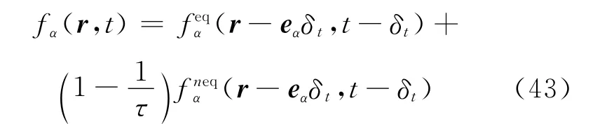
Furthermore，by substituting Eq.（38）into Eq.（43），we obtain

Equation（44）is actually equivalent to fα（r，t）＝r，t）＋（r，t）.Finally，Summation of Eq.（44）overαand applying the compatibility condition gives

Eqs.（45，46）show that the conservative flow variables at the cell interface are fully determined from the equilibrium distribution functions at the surrounding points.As equilibrium distribution functions only depend on the macroscopic flow variables，there is no need to store the densi－ty distribution functions for all the time levels.In fact，at any time step，we locally reconstruct a LBM solution at each cell interface independently.The reconstruction process is applied locally and repeated from one time level to another time level.Overall，the basic solution procedure of LBFS can be summarized below：

（1）At beginning，we need to choose a lattice velocity model such as D2Q9model.Then we need to specify a streaming time stepδt.The choice ofδtshould satisfy the constraint that the location of（r－eαδt）must be within either the cell Ωior the cellΩi＋1.Note that as local LBM solution is reconstructed at each cell interface，different interfaces could use differentδt.This provides agreat flexibility for application if we use non－uniform mesh or solve problems with a curved boundary.Onceδtis chosen，the single relaxation parameterτin LBFS is calculated by Eq.（28）.

（2）For the considered interface position r，identify its surrounding positions（r－eαδt），and then use Eqs.（39，40）to compute the macroscopic flow variables at those positions.

（3）Use Eq.（27）to calculate the equilibrium density distribution function（r－eαδt，t－δt）.

（4）Compute the macroscopic flow variables at the cell interface by using Eqs.（45）and（46），and further calculate（r，t）by Eq.（27）.

（6）Compute the fluxes at the cell interface by Eq.（36）.

（7）Once fluxes at all cell interfaces are obtained，solve ordinary differential Eq.（34）by using 4－stage Runge－Kutta scheme.

It is indicated that the present LBFS can be used to simulate both incompressible viscous flows and incompressible inviscid flows.For the inviscid flow，we just simply setτ＝0.5.Another point to note is that the time marching step used in solving Eq.（34）and the streaming time stepδtused in LBFS are independent.δtcan be selected differently at different interface and dif－ferent time level.Numerical experiments show thatδthas no effect on the solution accuracy.

4 Numerical Examples and Discussion

In this section，the developed LBFS is validated by its application to solve some test problems.In all following simulations，the non－free parameter D1Q4model［33－34］is used for simulation of compressible inviscid flows，and the D2Q9lattice velocity model is applied for simulation of two－dimensional incompressible viscous flows.

4.1 Simulation of two－dimensional compressible inviscid flows

At first，the LBFS developed in Section 2 will be applied to simulate three two－dimensional compressible inviscid flows.They are the flow around a NACA0012airfoil，the flow around a forward facing step，and the flow around a circular cylinder.For the flow around the NACA0012airfoil，the free－stream Mach number is taken as 0.8 and the angle of attack is chosen as 1.25°.Unstructured grid with 10 382cells is used for numerical computation.Both LBFS and Roe scheme are applied to solve this problem on the same computational mesh.It was found that the pressure coefficient distributions obtained by LBFS and Roe scheme are close to each other.The lift and drag coefficients（Cland Cd）obtained by LBFS are respectively 0.304 1and 0.023 7，which agree well with the results given from Roe scheme（Cl＝0.283 6，Cd＝0.021 5）and those of Stolcis and Johnston［35］（Cl＝0.339 7，Cd＝0.022 8）.Fig.5shows the pressure contours around the airfoil.As can be seen clearly，the shock wave on the upper surface is well captured by present solver.The second test example in this part is a stationary flow（Mach number equals 3）hitting a rectangular step.This problem has been well studied by Woodward and Colella［36］，and is often used to investigate performance of new numerical methods for capturing the shock waves.In our computation，a uniform mesh size of 300×100is used.Fig.6shows the density contours computed by present solver.Our results are in good agreement with those in Ref.［36］.It is noted that no special treatment around step corner is made in the present computation，which is often needed by conventional schemes.To further explore the capability of present solver for simulation of hypersonic flows with strong shock waves，the flow around a circular cylinder is simulated.For this case，a uniform mesh size of 160×40in the cylindrical coordinate system is used.It is well known that for this problem，conventional numerical schemes such as Roe scheme may encounter the″carbuncle phenomenon″in front of cylinder when the free stream Mach number is high.The″carbuncle phenomenon″may be due to unsatisfying of entropy condition and negative value of density in the local region.We have used different free－stream Mach numbers to test simulation of this problem by LBFS.For all the cases tested（free－stream Mach number up to 100），no″carbuncle phenom－enon″was found in the present results.This can be seen clearly from Fig.7，which shows pressure contours of Ma＝3and 100.Both results show regular pressure distribution around the cylinder.

Fig.5 Pressure contours around NACA0012airfoil

Fig.6 Density contours for flow around a forward facing step

Fig.7 Pressure contours for flow around a circular cylinder

4.2 Simulation of compressible inviscid flows around ONERA M6wing

Fig.8 Partial view of computational mesh for flow around ONERA M6wing

To investigate the capability of present LBFS for solving practical flow problems，the threedimensional（3D）transonic flow around the ONERA M6wing is simulated.This is also a standard test case for 3Dcomputations.For numerical simulation，the free－stream Mach number is taken as 0.839 5and the angle of attack is chosen as 3.06°.The part of computational mesh is shown in Fig.8，which has 294 912cells.The pressure contours obtained by present solver are displayed in Fig.9.The″λ″shape shock wave on the upper surface of the wing can be seen clearly in Fig.9，which is in line with the result in Ref.［37］.The pressure coefficient distribution at a section of z／b＝0.65is shown in Fig.10.Also included in Fig.10are the experimental data given in Ref.［38］.As can been clearly，the present results quantitatively compare very well with the experimental data.

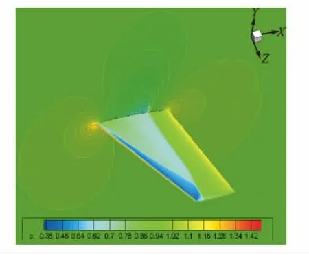
Fig.9 Pressure contours around ONERA M6wing

Fig.10 Pressure coefficient distribution at section of z／b＝0.65on M6wing

4.3 Simulation of incompressible lid－driven flow in a square cavity

The lid－driven flow in a square cavity is a standard test case for validating new numerical methods in simulation of incompressible viscous flows.The flow pattern of this problem is governed by the Reynolds number defined by Re＝UL／ν，where Uis the lid speed，Lis the length of the cavity，andνis the kinematic viscosity of fluid.Two cases of this problem at moderate and high Reynolds numbers of 3 200and 7 500are considered in this work.LBFS introduced in Section 3will be applied to solve this problem and the following problems.

To conduct numerical simulations，the nonuniform grid is generated according to the following formulation

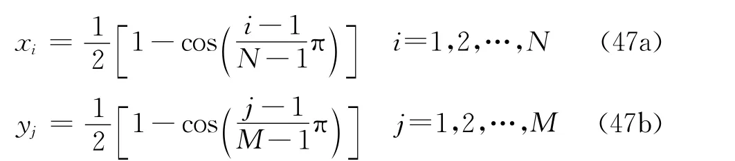
where Nand Mare the total number of mesh points in the xand ydirections respectively.With Eq.（47），the non－uniform grids of 101×101for Re＝3 200and 121×121for Re＝7 500are used respectively.In the present study，we set U＝0.1 and L＝1.The initial flow field is at rest.

Table 1compares the locations of the primary vortex centers at Re＝3 200and 7 500obtained by LBFS with those given by Ghia et al［39］.As can be seen，the maximum relative error between present results and those of Ghia et al［39］is less than 1.1%.Fig.11displays u－velocity profile along the horizontal centerline and v－velocity profile along the vertical centerline of the considered two cases.As can be seen from this figure，the present results agree very well with those of Ghia et al［39］.Fig.12shows the streamlines of Re＝3 200，7 500.The most striking aspect of this figure is that the Reynolds number apparently has unique effect on flow patterns.Secondary and tertiary vortices appear and evolve into larger ones as Re becomes large.These results and observations are in good agreement with those of Ghia et al［39］.

Table 1 Locations of primary vortex centers at different Reynolds numbers

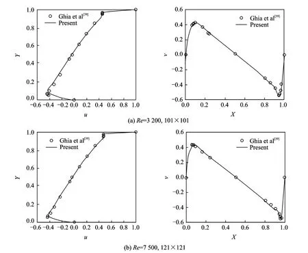
Fig.11 uand vvelocity profiles along horizontal and vertical centerlines for a lid－driven cavity flow at Re＝3 200，7 500

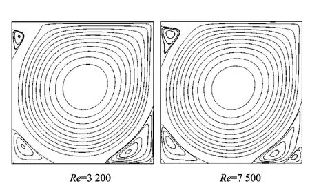
Fig.12 Streamlines of a lid－driven cavity flow at Re＝3 200，7 500

Note that for this test example，we have also studied the effect of streaming distance in local reconstruction of LBM solution.It was found that when the streaming distance is less than half of mesh spacing in the two neighboring cells（this constraint guarantees that only interpolation is performed in each cell），any value of streaming distance will have no effect on the accuracy of solution.This is an appealing feature，which ensures that LBFS can be easily applied on non－uniform mesh.

4.4 Simulation of incompressible polar cavity flow

Although the complex lid－driven cavity flows have been successfully simulated to validate the present solver，the geometry of the cavity which only involves straight boundaries is nevertheless simple.To further illustrate the capability of LBFS for problems with curved boundary，apolar cavity flow is simulated on body－fitted meshes.The schematic diagram and the typical non－uniform mesh for this problem are depicted in Fig.13.As shown in Fig.13，a sector with an angle ofθ＝1is bounded by two straight walls and two curved walls with radii of Riand Ro.The inner curved wall rotates with an azimuthal velocity of Uθ.The flow pattern of this problem is governed by the Reynolds number defined as Re＝UθRi／ν.In this study，two cases of Re＝60and 1 000are considered，and the following parameters are applied：Ri＝1.0，Ro＝2.0，ρ0＝1.0and Uθ＝0.1.Initially，the flow field is at rest.Fig.14shows the radial（ur）and azimuthal（uθ）velocity profiles along the horizontal line ofθ＝0.5at Re＝60and 1 000.The experimental results of Fuchs and Tillmark［40］and the numerical solutions of Shu et al［41］obtained by applying Taylor series expansion－and least－square－based LBM（TLLBM）are also included for comparison.Note that the present results and TLLBM results are both obtained on the same non－uniform grids，i.e.，61×61for Re＝60and 81×81for Re＝1 000.It can be seen that good agreements have been achieved between the present results and those of Fuchs and Tillmark［40］and Shu et al［41］，which validate the reliability of the present solver for problems with curved boundary and use of non－uniform grid.The streamlines are shown in Fig.15.As can be seen，with increase of the Reynolds number，the primary vortex moves upward and reduces its size.At the same time，the two secondary vortices at the upper－right and lower－right corners enlarge their size.These observations agree well with those of Fuchs and Tillmark［40］.

Fig.13 Schematic diagram and a typical body－fitted mesh for flow in a polar lid－driven cavity

4.5 Simulation of flow induced by an impulsively started cylinder

In this part，LBFS is applied to simulate the unsteady flow induced by an impulsively started circular cylinder.The Reynolds number of this flow is defined as Re＝UD／ν，where Uis the freestream velocity and Dis the diameter of cylinder.A wide range of Reynolds numbers from 102to 104are considered in this study to further demonstrate the capability of LBFS for effective simula－tion of unsteady flows at high Reynolds numbers.

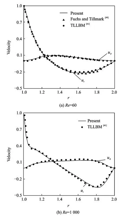
Fig.14 Comparison of radial（ur）and azimuthal（uθ）velocity profiles along the horizontal line of θ＝0.5for the polar cavity flow

Fig.15 Streamlines for the polar cavity flow at Re＝60and 1 000

In the present simulation，for flows at Re＝550and 3 000，a mesh size of 301×201is used and the outer boundary is placed at 15diam－eters away from the cylinder center.For the flow at Re＝9 950，the computational mesh is set as 301×351and the outer boundary is set as 4diameters away from the cylinder center.The flow parameters are set as：ρ＝1.0，U＝0.1and a＝0.5.Initially，the flow field is at rest.

For incompressible flows around the circular cylinder at high Reynolds number，apair of primary symmetric vortices will be developed at the rear of cylinder initially.With increase of the Reynolds number，the size of the two vortices is decreased.As time increases，the primary vortices will move away and detach from the rear of cylinder.In the meantime，apair of secondary symmetric vortices appears and becomes larger and stronger.The vortex structures exhibit the so－called″α″and″β″patterns.All these features have been well captured in present simulation.To save the space，these results are not displayed in this paper.Fig.16shows a quantitative comparison of the time evolution of the vortex length with experimental data of Bouard and Coutanceau［42］.Obviously，good agreement has been achieved.For Re＝550，the vortex length almost grows linearly with respect to time.For high Reynolds numbers（Re＝3 000and 9 500），a slow increase in vortex length，which corresponds to the″fore－wake″region，can be observed when t＜3.0s.When t＞3s，a fast growth of the vortex length can be seen due to destruction of the″fore－wake″.Fig.17further compares the radial velocity along the symmetric axis at Re＝3 000with experimental data of Bouard and Coutanceau［42］and numerical results of Niu et al［43］.Once again，good agreement is achieved.

Fig.16 Comparison of the vortex length for flow induced by impulsively started cylinder at different Reynolds numbers

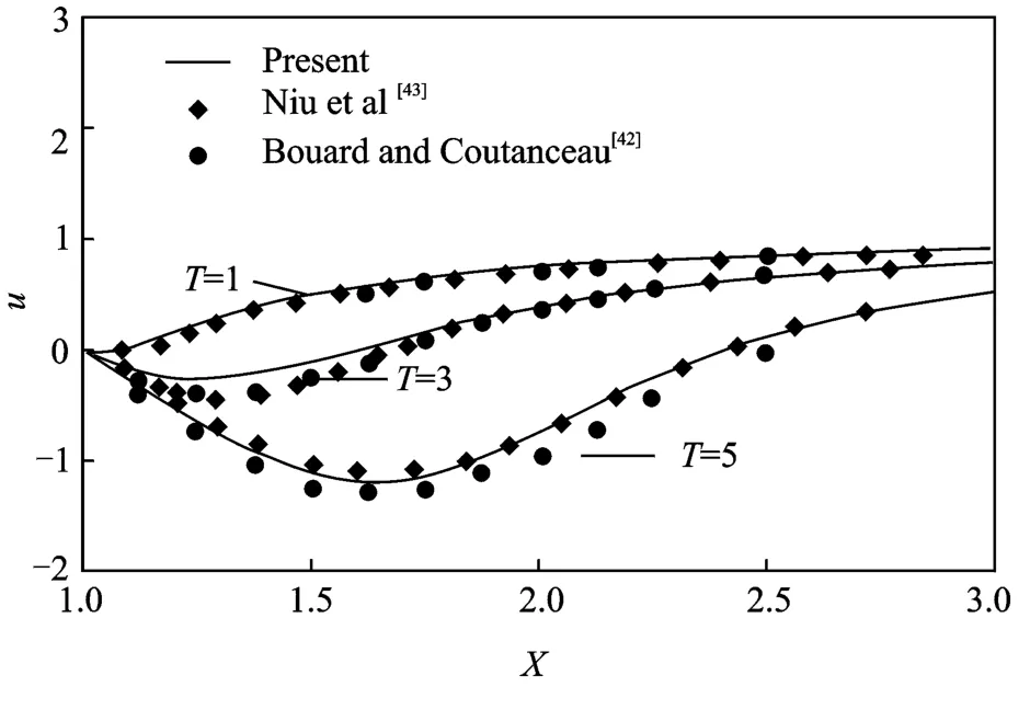
Fig.17 Comparison of the radial velocity along symmetric axis for flow induced by impulsively started cylinder at Re＝3 000

5 Conclusions

In this paper，the LBFS is presented for simulation of compressible and incompressible flows.The solver is based on numerical discretization of FVM to the governing differential equations（Navier－Stokes equations or Euler equations）.Specifically，the conservative flow variables at cell centers are given from the solution of discrete governing equations but numerical fluxes at cell interfaces are evaluated by local reconstruction of LBE solution from flow variables at cell centers.Two versions of LBFS are presented in this paper.One is to locally apply 1Dcompressible LB model along the normal direction to the cell interface for simulation of compressible inviscid flows.The other is to locally apply incompressible LB model at the cell interface for simulation of incompressible viscous flows.

The present LBFS is well validated by its application to simulate some two－and three－dimensional compressible inviscid flows，and twodimensional incompressible viscous flows.Numerical results show that the compressible version of LBFS can well simulate compressible inviscid flows with strong shock waves，and its incom－pressible version can accurately simulate incompressible viscous flows with curved boundary and non－uniform mesh.It removes the drawbacks of conventional LBM such as limitation to the uniform mesh，tie－up of mesh spacing and time interval.It is believed that LBFS has a great potential for solving various flow problems in practice.

［1］ Roach P J.Computational fluid dynamics［M］.Hermosa Beach，USA：Hermosa Press，1972.

［2］ Anderson D A，Tannehill J C，Pletcher R H.Computational fluid mechanics and heat transfer［M］.New York，USA：McGraw－Hill，1984.

［3］ Hirsch C.Numerical computation of internal and external flows［M］.Hoboken，USA：John Wiley ＆Sons，1988.

［4］ Fletcher C A J.Computational techniques for fluid dynamics：fundamental and general techniques［M］.Berlin，Germany：Springer－Verlag，1991.

［5］ Anderson J D.Computational fluid dynamics：the basics with applications［M］.New York，USA：McGraw－Hill，1995.

［6］ Versteeg H K，Malalasekera W.An introduction to computational fluid dynamics：the finite volume method［M］.Harlow，England：Longman Scientific＆Technical，1995.

［7］ Donea J，Huerta A.Finite element methods for flow problems［M］.Hoboken，USA：John Wiley，2003.

［8］ Wendt J F.Computational fluid dynamics［M］.Berlin，Germany：Springer Berlin Heidelberg，2009.

［9］ Funaro D.Polynomial approximation of differential equations［M］.Berlin，Germany：Springer－Verlag，1992.

［10］Buhmann M D.Radial basis functions：theory and implementations［M］.Cambridge University Press，2003.

［11］Godunov S K.A difference method for numerical calculation of discontinuous solutions of the equations of hydrodynamics［J］.Matematicheskii Sbornik，1959，47：271－306.

［12］Roe P L.Approximate Riemann solvers，parameter vectors，and difference schemes［J］.Journal of Computational Physics，1981，43：357－372.

［13］Steger J，Warming R.Flux vector splitting of the inviscid gas dynamic equations with applications to finite－difference methods［J］.Journal of Computational Physics，1981，40：263－293.

［14］Shu C W，Osher S.Efficient implementation of es－sentially non－oscillatory shock－capturing scheme［J］.Journal of Computational Physics，1988，77：439－471.

［15］Shu C W.High order weighted essentially non－oscillatory schemes for convection dominated problems［J］.SIAM Review，2009，51：82－126.

［16］B van Leer，Lo M.A discontinuous Galerkin method for diffusion based on recovery［J］.Journal of Scientific Computation，2011，46：314－328.

［17］Xu K.A gas－kinetic BGK scheme for the Navier－Stocks equations and its connection with artificial dissipation and Godunov method［J］.J Comput Phys，2001，171：289－335.

［18］Chen S Z，Xu K，Lee C B，et al，A unified gas kinetic scheme with moving mesh and velocity space adaptation［J］.Journal of Computational Physics，2012，231：6643－6664.

［19］Yang L M，Shu C，Wu J，et al.Circular functionbased gas－kinetic scheme for simulation of inviscid compressible flows［J］.J Comput Phy，2013，255：540－557.

［20］Chen S，Chen H，Martínez D，et al.Lattice Boltzmann model for simulation of magnetohydrodynamics［J］.Phys Rev Let，1991，67（27）：3776－3779.

［21］Qian Y H，D′Humières D，Lallemand P.Lattice BGK models for Navier－Stokes equation［J］.Europhys Lett，1992，17：479－484.

［22］Chen S，Doolen G.Lattice Boltzmann method for fluid flows［J］.Ann Rev Fluid Mech，1998，30：329－64.

［23］Mei R，Luo L S，Shyy W.An accurate curved boundary treatment in the lattice Boltzmann method［J］.J Comput Phys，1999，155：307－330.

［24］Guo Z L，Shi B C，Wang N C.Lattice BGK model for incompressible Navier－Stokes equation［J］.J Comput Phys，2000，165：288－306.

［25］Shu C，Chew Y T，Niu X D.Least square－based LBM：a meshless approach for simulation of flows with complex geometry［J］.Phys Rev E，2001：64，045701.

［26］Shu C，Niu X D，Chew Y T.Taylor series expansion－and least square－based lattice Boltzmann method：two－dimensional formulation and its applications［J］.Phys Rev E，2002，65：036708.

［27］Succi S，Mesoscopic modeling of slip motion at fluidsolid interfaces with heterogeneous catalysis［J］.Phys Rev Lett，2002，89：064502.

［28］Shan X，Yuan X F，Chen H.Kinetic theory representation of hydrodynamics：A way beyond the Navi－er－Stokes equation［J］.J Fluid Mech，2006，550：413－441.

［29］Guo Z L，Asinari P，Zheng C G.Lattice Boltzmann equation for microscale gas flows of binary mixtures［J］.Phys Rev E，2009，79：026702.

［30］Aidun C K，Clausen J R.Lattice－Boltzmann method for complex flows［J］.Ann Rev Fluid Mech，2010，42：439－72.

［31］Wu J，Shu C.A solution－adaptive lattice Boltzmann method for two－dimensional incompressible viscous flows［J］.J Comput Phys，2011，230：2246－2269.

［32］Guo Z，Shu C.Lattice Boltzmann method and its applications in engineering［J］.World Scientific Publishing，2013.

［33］Yang L M，Shu C，Wu J.Development and comparative studies of three non－free parameter lattice Boltzmann models for simulation of compressible flows［J］.Adv Appl Math Mech，2012，4：454－472.

［34］Yang L M，Shu C，Wu J.A moment conservationbased non－free parameter compressible lattice Boltzmann model and its application for flux evaluation at cell interface［J］.Comput Fluids，2013，79：190－199.

［35］Stolcis L，Johnston L J.Solution of the Euler equations on unstructured grids for two－dimensional compressible flow［J］.Aeronautical Journal，1990，94：181－195.

［36］Woodward P，Colella P.The numerical simulation of two－dimensional fluid flow with strong shocks［J］.Journal of Computational Physics，1984，54：115－173.

［37］Batina J T.Accuracy of an unstructured－grid upwind－Euler algorithm for the ONERA M6wing［J］.J Aircraft，1991，28：397－402.

［38］Schmitt V，Charpin F.Pressure distributions on the ONERA－M6－wing at transonic Mach numbers，experimental data base for computer program assessment［J］.Report of the Fluid Dynamics Panel Working Group 04，1979，AGARD AR：138.

［39］Ghia U，Chia K N，Shin C T.High－resolutions for incompressible flow using the Navier－Stokes equations：a multigrid method［J］.J Comput Phys，1982，48：387－411.

［40］Fuchs L，Tillmark N.Numerical and experimental study of driven flow in a polar cavity［J］.Int J Num Methods in Fluids，1985，5：311－329.

［41］Shu C，Niu X D，Chew Y T.Taylor series expansion－and least square－based lattice Boltzmann method：two－dimensional formulation and its applications［J］.Phys Rev E，2002，65：036708.

［42］Bouard R，Coutanceau M.The early stage of development of the wake behind an impulsively started cylinder for 40＜Re＜104［J］.J Fluid Mech，1980，101：583－607.

［43］Niu X D，Chew Y T，Shu C.Simulation of flows around an impulsively started circular by Taylor series expansion－and least squares－based lattice Boltzmann method［J］.J Comput Phys，2003，188：176－193.