Detrended analysis of Reynolds stress in a decaying turbulent flow in a wind tunnel with active grids*

AHMAD Imtiaz

Shanghai Institute of Applied Mathematics and Mechanics, Shanghai University, Shanghai 200072, China

Department of Mathematics, University of Azad Jammu and Kashmir, Muzaffarabad 13100, Pakistan,

E-mail: rajaimtiazahmad@live.com

HUANG Yong-xiang (黄永祥), LU Zhi-ming (卢志明)

Shanghai Institute of Applied Mathematics and Mechanics and Shanghai Key Laboratory of Mechanics in Energy Engineering, Shanghai University, Shanghai 200072, China

Detrended analysis of Reynolds stress in a decaying turbulent flow in a wind tunnel with active grids*

AHMAD Imtiaz

Shanghai Institute of Applied Mathematics and Mechanics, Shanghai University, Shanghai 200072, China

Department of Mathematics, University of Azad Jammu and Kashmir, Muzaffarabad 13100, Pakistan,

E-mail: rajaimtiazahmad@live.com

HUANG Yong-xiang (黄永祥), LU Zhi-ming (卢志明)

Shanghai Institute of Applied Mathematics and Mechanics and Shanghai Key Laboratory of Mechanics in Energy Engineering, Shanghai University, Shanghai 200072, China

(Received April 5, 2013, Revised January 3, 2014)

Multi-scale properties of Reynolds stress in decaying turbulence in a wind tunnel with high Reynolds number are investigated. Two filtering techniques i.e., the zeroth-order and first-order detrending methods are applied to the two velocity components, where the local mean value (resp. local linear trend) is removed in the former (latter) technique. Some basic statistics for thirty measurements show that the variation is very large at first two locations and relatively small at last two locations. Moderately good power law is found for the mean value of local Reynolds stress at last three measurement locations with scaling exponents approximately being 1.0 and a dual power law exists for the mean value of standard deviation of local Reynolds stress at all four measurement locations with scaling exponents being 0.53 and 0.58 for zeroth- and first-order filtering respectively. Present results about local Reynolds stress are useful to build and evaluate the model of sub-grid Reynolds stress in large eddy simulations.

Reynolds stress, multi-scale analysis, detrended analysis, power law

Introduction

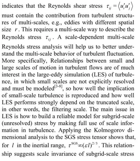
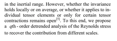
Fig.1 A 0.25 s portion of the measured longitudinal ()uand transverse ()vvelocity components. The local mean and linear trend for a window size =r0.05 s are also shown by thin solid line and thick solid line respectively

1. th-qorder detrended analysis

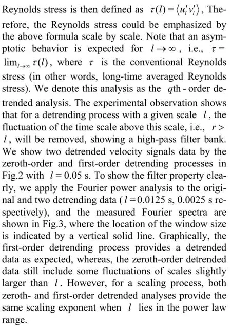
To show the multi-scale behavior of turbulent fluctuation, a 0.25 s portion of two velocity components from a decaying turbulent flow in a wind tunnel is shown in Fig.1 (see Section 2 for more detail). Visually, the longitudinal and transverse velocities are varying on different time scales, indicating the multiscale nature of the turbulent flow. They are positively correlated with each other on some portion and negatively on other portion. This could be shown more clearly by a linear trend fitting (bold black line) within a windowl=0.05 s. Note that the linear trend also shows positive correlation on some portion and negative on other portion.

Indeed, another version of detrended analysis, namely detrended fluctuation analysis (DFA), has been widely used for the analysis of a time series to characterize the scale invariance property. It wasproposed by Peng et al.[9]to characterize a scale invariance property of DNA sequence. Since its introduction, this method has been widely used in scale invariance analysis in a variety of fields[10-13]. It has been generalized to carry out cross correlation analysis by considering a similar fluctuation function between two variables[14]. Note that the difference between our proposal and the DFA is that the detrending procedure is directly performed on the original velocity signal without involving the so-called cumulative function. Another advantage of our proposal is that it keeps the same physical meaning as the original definition of the Reynolds stress.

Fig.2 An example of the qth-order detrending process, in which qth-order polynomial fitting within a window size l=0.05s is removed from the original velocity component. After the detrending process, the scale larger than the considered window size r＞l is expected to be removed

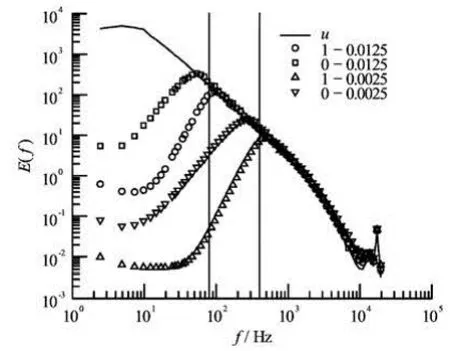
Fig.3 Measured Fourier power spectrum for the data with and without detrending process. The location of the window size is illustrated by a vertical line

Fig.4 Comparison of Fourier power spectral density E( f) for longitudinal (○) and transverse (□) velocity components at the measurement location x/ M=20. A power law behavior is observed on the range 20 Hz＜f＜1 000 Hz for both velocity components. The inertial range corresponds to a time range 0.001s＜t＜0.05s . For display clarity, the spectrum Ev(f) has been vertical shifted by multiplying a factor 4

2. Experimental data

We consider here a turbulent velocity database obtained from a decaying homogeneous and nearly isotropic turbulent flow in a wind tunnel, in which an active-grid technique is applied to achieve high Reynolds number. We use the data obtained at four downstream locationsx/M=20, 30, 40 and 48 respectively, whereMis the mesh size. The sampling frequency of HWA is 40 kHz and the measurement noise is aroundfN=20 kHz. The sampling time is 30 s foreach measurement and 30 measurements ofuandvcomponents are recorded at each location. So the total number ofu(resp.v) at each location is 30×1.2×106. Some parameters in this flow are listed in Table 1.

To determine the inertial range, we plot the Fourier power spectrumE(f) for the longitudinal and transverse velocity components measured at locationx/M=20 in Fig.4. A nearly two decades inertial range is found on the range 20 Hz＜f＜1000 Hz for both longitudinal and transverse velocity components respectively with scaling exponents 1.65 and 1.63. The observed inertial range corresponds to a time scale range 0.001s＜t＜0.05s. More detail about this experiment data base can be found in Ref.[15].

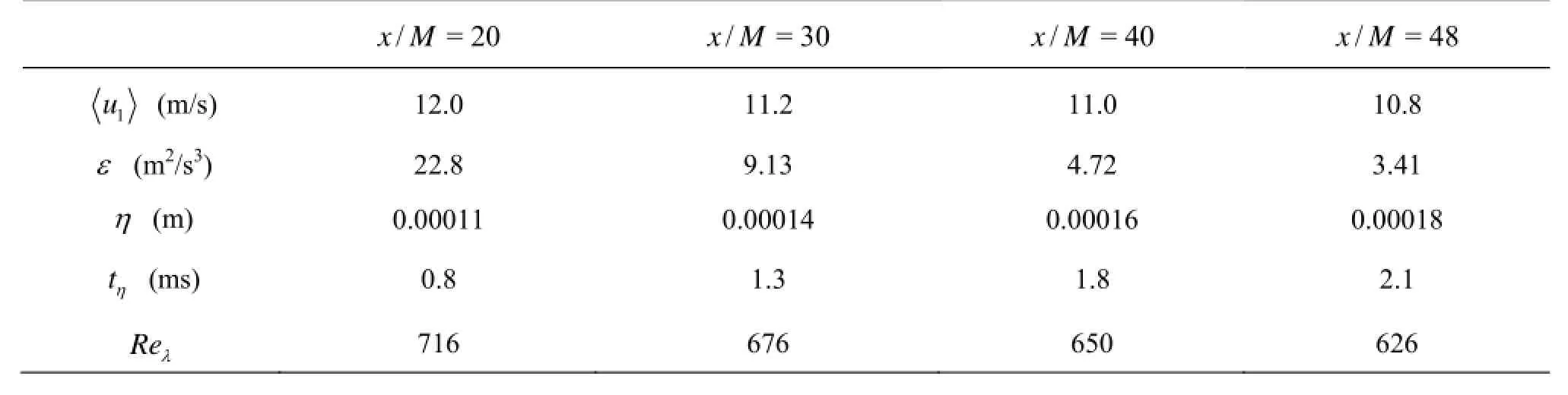
Table 1 Several parameters of the experiment data at four measurement locations

Fig.5 The mean velocity and Reynolds stress for 30 measurements at four streamwise locations

3. Results and discussion

Before analyzing the multi-scale behavior of the Reynolds stress, we investigate the variation of some fundamental statistics of velocity components for 30 measurements and the evolution of these statistics along four streamwise locations. As an example the streamwise evolution of mean velocities ofucomponent and the Reynolds stresses for 30 measurements are shown in Fig.5. It is clearly seen that the mean value of the Reynolds stress at the second location is much larger than the values at other three locations and the variation of mean velocity and Reynolds stress for 30 measurements at first two location is much larger than that at last two locations, which is due to smaller distance to the active grid at first two locations. Basic statistics of the velocity imply that the flows at last two locations are nearly stationary, homogeneous and isotropic. Now let us focus ourselves on the multiscale analysis of Reynolds stress.

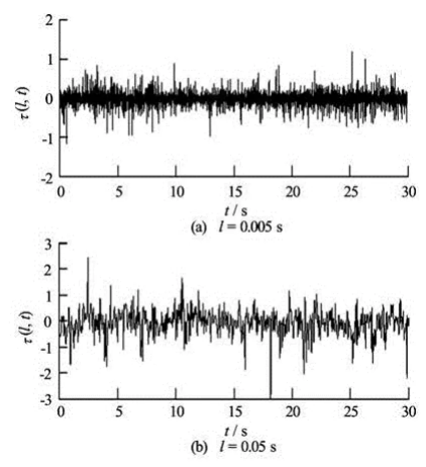
Fig.6 An example of the measured Reynolds stress ()lτ with two different slide windows

Figure 6 shows a 30 s of the measured ()lτusing the first-order detrend technique for (1) =l0.005 s(resp. 200 data points) and (2)l=0.05 s (resp. 2 000 data points) atx/M=48 without overlap. It is noted that two window sizes are within sub-inertial range, and the fluctuation is surprisingly large. Now we investigate the window sizeldependence of the mean value of the Reynolds stress and its standard deviation. The mean value is first calculated by averaging the time series ofτ(l) andσ(l) within one measurement, then averaging for 30 measurements. The mean values(l) of measuredτ(l) are shown in Fig.7. Shown in (a) is the Reynolds stress calculated with conventional way, i.e., local mean value is removed in theuandvvelocity components (with the zeroth-order detrended method), whereas shown in (b) is the one calculated with the first-order detrended method, i.e., the local linear trend is removed in theuandvvelocity components. As was expected, the results by two methods agree well whenlis large and the difference at smalllis obvious. Except for the first measurement locationx/M=20, a nearly three decades power-law behavior, i.e.,(l)～lα, is observed from the dissipation range to the inertial range, and the scaling exponents are about 1.00±0.05 for the zeroth-order detrending method, while the power-law is less satisfactory for the first-order detrending technique. The reason for this is unclear and needs further investigation. It is also observed from Fig.7 that whenlincreases, i.e., larger and larger scales are included, the measured Reynolds stress asymptotically approaches to the real one, i.e.,τ=liml→∞(l). The measuredτat the second location is 0.35, about 50% larger than those measured at the other 3 locations, which is 0.23± 0.04. The reasons why the first location is an exceptional one for the profile(l) and the second location is an exceptional one for the Reynolds stress are unclear since the active-grid technique is applied to obtain the high Reynolds number flow.

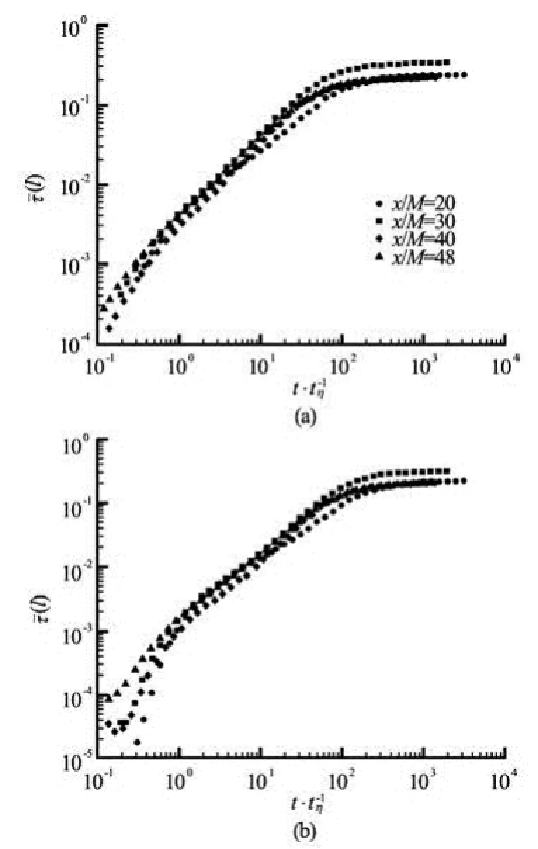
Fig.7 Experimental mean(l) for the measurement location. A nearly three-decade power law behavior, i.e.,(l)～lα, is observed on the range 0.5≤l/ tη＜100

Fig.8 Measured standard deviation ()lσ of ()lτ for four measurement locations. Two power-law behaviors are observed with a typical separation scale /l tη⋍100

Now let us consider the standard deviationσ(l) ofτ(l) by two methods at four locations, which is shown in Fig.8. It is seen that the measuredσ(l) is decreasing with flow development of stream-wise direction, and a dual power-law behavior is observed for all measurement locations. i.e., the standard deviation increases with the increase of window size and reaches the maximum value atl/tη～100 and then decreases gradually with the increase ofl. It is shown that a perfect power-law exists for all four locations and scaling exponents are the same also for four locations. To see this clearly we normalize theσ(l) by the corresponding maximum value and the time by thevalue where maximum value is reached. Figure 9 shows the normalized standard deviation of the Reynolds stress, and now four lines collapse surprisingly well for the first power law range. The scaling exponent is 0.53 and 0.58 for the zeroth- and firstorder detrending method respectively.

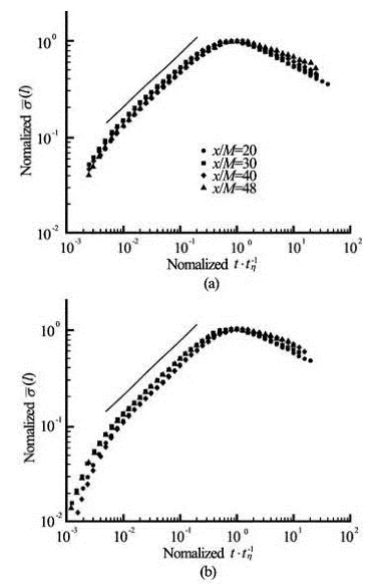
Fig.9 Rescaled σ(l). Power law behavior is observed on a normalized range 0.01≤l/ tp≤0.1 with scaling exponents 0.53±0.02 and 0.58±0.02

4. Conclusions and discussion

Acknowledgment

We thank Prof. Meneveau for sharing his experimental velocity database, which is available for download at Meneveau’s web page: http://www.me.jhu. edu/meneveau/datasets.html.

[1] FRISCH U. Turbulence: The Legacy of A. N. Kolmogorov[M]. Cambridge, UK: Cambridge University Press, 1995.

[2] POPE S. B. Turbulent flows[M]. Cambridge, UK: Cambridge University Press, 2000.

[3] MENEVEAU C., KATZ J. Scale-invariance and turbulence models for large-eddy simulation[J]. Annual Review Fluid Mechanics, 2000, 32: 1-32.

[4] SPALART P. R. Strategies for turbulence modeling and simulation[J]. International Journal of Heat and Fluid Flow, 2000, 21(3): 252-263.

[5] POPE S. B. Ten questions concerning the large-eddy simulation of turbulent flows[J]. New Journal of Physics, 2004, 6(35): 1-23.

[6] DAI Zheng-yuan. The filtering mesh scale in the largeeddy simulation and its application[D]. Doctoral Thesis, Shanghai, China: Shanghai Jiao Tong University, 2007(in Chinese).

[7] ZHANG Bin, WANG Tong and GU Chuan-gang. An adaptive control strategy for proper mesh distribution in large eddy simulation[J]. Journal of Hydrodynamics, 2010, 22(6): 865-870.

[8] CHEN S., XIA Z. and RUI S. et al. Reynolds-stressconstrained large-eddy simulation of wall-bounded turbulent flow[J]. Journal of Fluid Mechanics, 2012, 703: 1-28.

[9] PENG C. K., BULDYREV S. V. and HAVLIN S. et al. Mosaic organization of DNA nucleotides[J]. Physical Review E, 1994, 49(2): 1685-1689.

[10] HENEGHAN C., MCDARBY G. Establishing the relation between detrended fluctuation analysis and power spectral density analysis for stochastic processes[J].Physical Review E, 2000, 62(5): 6103-6110.

[11] ZHANG Q., XU C. and CHEN Y. et al. Multifractal detrended fluctuation analysis of streamflow series of the Yangtze River basin, China[J]. Hydrological Processes, 2008, 22(26): 4997-5003.

[12] BARDET J., KAMMOUN I. Asymptotic properties of the detrended fluctuation analysis of long-range dependent processes[J]. Information Theory, IEEE Transactions on, 2008, 54(5): 2041-2052.

[13] KANTELHARDT J., ZSCHIEGNER S. and KOSCIELNY-BUNDE E. et al. Multifractal detrended fluctuation analysis of nonstationary time series[J]. Physica A, 2002, 316(1-4): 87-114.

[14] KRISTOUFEK L., Multifractal height cross-correlation analysis: A new method for analyzing long-range crosscorrelations[J]. Europhysics Letters, 2011, 95(6): 68001.

[15] KANG H., CHESTER S. and MENEVEAU C. Decaying turbulence in an active-grid-generated flow and comparisons with large-eddy simulation[J]. Journal of Fluid Mechanics, 2003, 480: 129-160.

10.1016/S1001-6058(14)60014-7

* Project supported by the National Natural Science Foundation of China (Grant Nos. 11272196, 11202122), the Key Project of Shanghai Municipal Education Commission (Grant No. 11ZZ87) and the Shanghai Pujiang Project (Grant No. 12PJ1403500).

Biography: AHMAD Imtiaz (1974-), Male, Ph. D.

HUANG Yong-xiang,

E-mail: yongxianghuang@gmail.com