Hydroacoustic analysis of open cavity subsonic flow based on multiple parameter numerical models*

YUAN Guo-qing （袁国清）， JIANG Wei-kang （蒋伟康）， HUA Hong-xing （华宏星）

State Key Laboratory of Mechanical System and Vibration， Shanghai Jiao Tong University， Shanghai 200240，China， E-mail: yuan_weizhao@163.com

Hydroacoustic analysis of open cavity subsonic flow based on multiple parameter numerical models*

YUAN Guo-qing （袁国清）， JIANG Wei-kang （蒋伟康）， HUA Hong-xing （华宏星）

State Key Laboratory of Mechanical System and Vibration， Shanghai Jiao Tong University， Shanghai 200240，China， E-mail: yuan_weizhao@163.com

2015，27（5）:668-678

The prediction of the flow-induced noise level is a key issue in the fluid-dynamic acoustics. In the hydroacoustics field，the complicated feedback induced by the flow past open cavities can amplify the convection instability in the shear layer which further leads to important noise radiations. The noise consists of intense narrowband and broadband components. In this paper， the level of the noise radiated by a subsonic cavity flow is calculated by using numerical flow computations based on the large eddy simulation （LES） and by solving the Ffowcs Williams-Hawkings equation. A series of three-dimensional open cavity models with overset grids and appropriate boundary conditions are developed for the hydroacoustic numerical computation. The self-sustained oscillation characteristics of the cavity flow are investigated， together with the mechanisms of the cavity noise generation. The distinguishing features of the flow-induced noise of the underwater structure cavities are studied with respect to the parameters of the cavity models， such as the free stream velocity， the dimensions of the cavity mouth， the angle of the cavity neck， the horizontal and vertical porous cavity models and the actual submarine open cavity model with an incoming flow attack angle. It is shown that it may be feasible to reduce the flow-induced noise by appropriate optimal parameters of the underwater structure cavities.

flow-induced noise， underwater structure cavity， large eddy simulation （LES）， Ffowcs Williams-Hawkings equation

Introduction

The prediction of the flow-induced noise level［1，2］is an important and complex issue in the fluid-dynamic acoustics field. Hydroacoustics is not a much studied field. Generally speaking， the hydroacoustics problem features a low acoustic conversion efficiency，a low Mach number and a high Reynolds number. The prediction of hydroacoustics requires a coupling analysis of the sound and the structure. Therefore， it is more difficult than the prediction in aeroacoustics.

Since the subsonic speed of the water flow is very low compared with the high speed of the air flow，the acoustic wavelength exceeds any characteristic dimension of the cavity. The flow Mach number is close to the incompressible flow limit， so the coupling effect between the hydrodynamic field and the sound field can be ignored. A splitting approach can， therefore， be employed， which is to decompose the hydroacoustics problem into an incompressible flow problem and an acoustic one. For a given flow， with the specification of the appropriate initial and boundary conditions， the hydrodynamic field is solved numerically. Generally speaking， there are three numerical simulation approaches， which are the direct numerical simulations（DNS）［3，4］， the Reynolds averaged Navier-Stokes（RANS） simulations［5，6］and the large-eddy simulations （LES）［7，8］. In view of the high Reynolds number and the low Mach number， the LES can achieve a balance between the computational cost and the sufficient turbulent features. In the acoustic field， the acoustic analogy was built by Lighthill （Lighthill equation），Curle， Ffowcs Williams and Hawkings （FW-H equation）， and was extended by Casalino［9］， Ask and Davidson［10］and Spalart［11］. The FW-H equation is an inhomogeneous wave equation with three acoustic source terms to be determined by the hydrodynamic field calculation， and to include the effects of the solid surfaces in an arbitrary motion. For a moving underwater structure cavity， the FW-H acoustic analogy me-thod has advantages in the sound field numeral calculation. Briefly， the splitting approach for the open cavity subsonic flow is a hybrid LES-FW-H method proposed by Wang and Wang［12］， Zhang et al.［13］and Zhang et al.［14］.

The flow-induced noise of an open cavity is the dominant part of the noise radiated by the moving underwater structure［15-17］. In the present study， the level of the noise radiated by a subsonic cavity flow is calculated with the mentioned splitting method. The hydrodynamic field is solved by using the Large-eddy simulation and the dipole source of the structure wall is obtained. After that， the sound field is solved by using the FW-H acoustic analogy and the flow-induced noise level of cavities is obtained. Three-dimensional open cavity models are established for the hydroacoustics numerical computation. The self-sustained oscillations of the cavity flow are investigated， together with the mechanisms for the cavity noise generation.

1. Numerical methods

1.1 Large-eddy simulation

Nearly all computational cost of the DNS is expended on the smallest scale motions， whereas the flow energy and the anisotropy are contained predominantly in the larger-scale motions. In the LES， the flow dynamics of the larger-scale motions are computed explicitly， while the influence of the smaller motions are represented by simple models. Thus， compared with the DNS， the vast computational effort of explicitly representing the small-scale motions is avoided， and a sufficient precision can be assured.

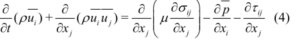
In the LES， the mesh grid cannot resolve all the scales of the flow. The governing equations are obtained after filtering. The scales larger than the filter width are computed explicitly， and the subgrid scales（SGS） are modelled. The filter functionG is defined and a flow variableφis filtered as:

whereV is the volume of the mesh，v is the flow field. Using the filter function， the continuity equation and the incompressible Navier-Stokes equations are obtained after filtering， as:

1.2 Acoustic analogy

The sound field radiated by the moving structure is evaluated using the Ffowcs Williams-Hawking integral equation. The FW-H equation is based on the continuity equation and the Navier-Stokes equations in the form of an inhomogeneous wave equation with two surface source terms and a volume source term. Using the impermeability condition on the surface of the moving structure， the density fluctuation FW-H equation is:

in which

ρ0is the density，Uiis the velocity，pijis the compressive stress tensor，c0is the velocity of sound，vnis the normal velocity of the surface node of the moving structure，Tijis the still Lighthill stress tensor，and the equation f=0defines the surface of the moving structure， outside of which the pressure field is calculated.

The FW-H acoustic analogy method has the following advantages. Firstly， on the right hand side of the equation， three sound source terms have clear physical meanings， which is very useful to understand the noise generation. The first monopole source term is the thickness noise source， which is completely determined by the geometry and the surface normal velocity of the moving structure. The second dipole sourceterm is the load force source， produced by the hydrodynamic effect on the structure surface. The third quadrupole source term is considered as the nonlinear effects， such as the nonlinear wave propagation， the changed local sound speed， the shock wave， the vortex and the changed turbulence. Secondly， the decomposition of three sound source terms has greatly facilitated the numerical calculation since by that means， not all three source terms need to be considered in acoustic problems. Especially in the case of water flow with low Mach number， the third quadrupole source makes a very small contribution to the field and can be neglected. In addition， as the surface normal velocity of the moving structure generally is a constant and the acoustic radiation of the first monopole source is very small， the second dipole source is the principal sound source and deserves a special attention. Finally， the fluid-dynamic acoustics calculation procedures based on the FW-H equation are very well-studied， we have the CFD softwares such as: the Ansys CFX， the Fluent and the acoustic calculation softwares such as: the LMS sysnoise， the LMS virtual lab. In engineering practices for the aeroacoustic problem， these numerical algorithms were verified as stable， reliable and accurate methods. of the actual submarine open hole models （Models V）are included in the study of the flow-induced noise，which are as follows:

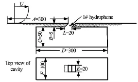
Fig.1 Sketch of underwater structure open cavity

Models I: To study the effects of the free stream velocity， where different flow velocities: 2.5 m/s，5 m/s， 10 m/s and 20 m/s are applied. And the effects of the boundary layer thickness are considered by extending the upstream solid wall of the cavity.

Models II: The shapes of hole （i.e.， circle， square，rectangle and rhombus） and the geometrical dimensions （i.e.， aspect ratio ζ=0.5， 1， 2， 4） are used to study the effect of the hole parameters on the flow-induced noise.

Models IIII: Considering the impingement of the vortical perturbations on the downstream corner， a series of hole neck angles （i.e.，15o，30o，45o，60o，75o，90o） are used.

Models IV: Considering the flow-induced noises of the porous cavity models， the horizontal and vertical porous cavities （i.e.， 1， 2， 4， 8 holes） are used.

Models V: According to the actual submarine open holes， the 18 horizontal porous cavity model is established in order to analysis the frequency spectrums of the measurement points. And considering the angle between the incoming flow and the submarine tail， the flow-induced noise frequency spectrum of the attack angle model is discussed.

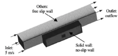
Fig.2 The meshes and boundary conditions of CFD

2. Underwater structure cavity computation models

2.1 Computation model

A schematic view of an underwater structure cavity is shown in Fig.1. In the simplified model， there is an oblique single square hole in an angleαat a plane. 1# hydrophone is located in the center of the hole to monitor the near-field hydroacoustics characteristics. In order to study the self-sustained oscillations of the cavity flow and the mechanisms of the cavity noise generation， a series of three-dimensional open cavity models are established based on the simplified model. From different aspects， the hydrodynamic field information （Models I）， the geometrical dimensions of the open cavity mouth （Models II and Models IIII）， the numbers of the horizontal and vertical porous cavities （Models IV） and the attack angles

2.2 Meshes and boundary conditions

The meshes and the boundary conditions of the CFD are shown in Fig.2. The CFD meshes include 1.8×106meshes of non-uniform size inside the fluid field with a mesh shrunk ratio near the wall. The first layer scale near the wall is 0.3 mm in order to catch the viscous stress change. In view of the gradient distribution of the flow field parameters， the much more coarse mesh size can be used in places away from the wall. This non-uniform size mesh method ensures the computational accuracy with an acceptable computational cost. The computational domain extends over 15Ldownstream domain to make sure a steady tail flow，15Lupstream domain to correspond to a certain boundary thickness，5L in transverse direction and 5L in height， whereLis the stream direction scale of the cavity mouth.

At the inlet boundary， a uniform normal velocity profile is defined with u=5m/s， whereas the outflow boundary condition is used with a relative pressurepref，static=0Paat the outlet. On all solid boundaries， the no-slip conditionsu=v=w=0are imposed， with∂p/∂n=0， where nis the direction normal to the solid surface. The free slip condition is applied at the other boundary of the fluid domain. In the fluid domain， the adiabatic condition and the incompressible condition are used in the calculation. The instantaneous computation time step is 5×10-4s， which corresponds to an analysis frequency up to 10 kHz.

Fig.3 The meshes and boundary conditions in acoustic field computation

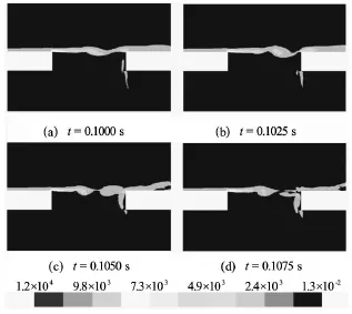
Fig.4 One period of vorticity distribution contours of stream direction slice

Because the acoustic computation is separated from the CFD， the acoustic field meshes and the acoustic boundary conditions should be defined additionally as shown in Fig.3. The acoustic field computation is based on the interior BEM frequency model. The acoustic meshes are built up from a coarse mesh size with 6k surface meshes， some parts of which is subdivided by considering the distribution of the surface dipole source. Non-reflecting conditions or absorbing boundary conditions are implemented by using the fluid impedance boundary on the other five surfaces so that out-going waves are not reflected into the computational domain. In the present study， the interior acoustic field scale is determined according to the flow field， but it can be arbitrary in some extent in theory.

3. Results and discussions

3.1 The vorticity field period and pressure feedback mechanism

One period of the vorticity distribution contours of a stream direction slice is shown in Fig.4. It is clearly identified by four steps. From Fig.4（a）， a vortex is generated and shed from the leading edge. This rolled-up vortex flows toward downstream in the next pictures， growing with convection along the distance downstream of the cavity leading edge （Fig.4（b））. When it travels close to the downstream edge， the incident vortex impinges on the trailing edge and it is split at its centre （Fig.4（c））. Part of the vortex escapes from the cavity and travels right along the flow direction， whereas the other part is rotated downwards into the cavity and rolls towards upstream （Fig.4（d））. Another vortex will be generated at the leading edge just like the one in Fig.4（a） and travels toward the trailing edge， sustaining the vortex impingement process. Then， a periodically oscillating flow over the cavity generates a self-sustained feedback loop and a tonal noise.

In this self-sustained feedback loop， the vortex energy is transformed into the acoustic energy by the vortex acceleration and deformation in the convection and impingement processes. The impingement of the vortex on the trailing edge produces a major pressure fluctuation， which propagates toward upstream in an acoustic wave style. Following the acoustic analogy theory， the surface dipole source generated in the impingement process is the principal sound source by comparing with the quadrupole vortex sound source generated in the convection process. Taking the surface dipole source as the only source term in the FW-H equation， the tonal noise radiated with the frequency of the self-sustained oscillation can be calculated easily.

In the aerodynamic field， this self-sustained mechanism can be seen as the self-excitation effect of the fluid flow in order to distinguish it from the other two types of coupling of the fluid oscillation in the cavity，i.e. the interaction between the fluid and the cavity acoustic mode or the elastic cavity wall. As a type of interaction between the fluid and the cavity acoustic mode， the cavity acoustic modes control the fluid oscillation. The cavity acoustic mode frequencies are only related with the sonic velocity and the cavity size. Usually， the underwater structure cavity acoustic mode frequencies are much higher than the upper limit frequency considered， then this oscillation formcan be ignored. As a type of interaction between the fluid and the elastic cavity wall， it is associated with the material properties of the cavity wall. In view of the rigid wall as is assumed here， this oscillation mechanism does not exist. In brief， the distinguishing feature of the self-sustained oscillation mechanism mainly depends on the free shear layer instability in a feedback loop.

Table 1 The open cavity hydroacoustics data for different incoming flow velocity models

The oscillation period can be expressed as the time of a single vortex moving from the leading edge to the trailing edge and the time of the disturbance sound wave propagating from the trailing edge to the leading edge， as

The self-excited oscillation frequency can be obtained by the reciprocal of the right hand side of the equation， as

And the harmonic frequencies can be expressed as

where Ucis the convection velocity，Mac=Uc/c0is the convection Mach number. In the above equation，some inaccuracy is due to not considering the local sonic velocity and the recirculation vortex inside the cavity. For the problem of the flow over the open cavity of an underwater structure， a semi-empirical formula by Spalartb［11］can be used， where the Strouhal number is obtained as whereL is the stream direction scale of the cavity mouth，M∞is the mach number，a =0.25and kc=0.57. Using the above equation， the fundamental frequency isf1=106Hzat L =0.02m，U= 5 m/s.

3.2 Effects of free stream velocity and boundary layer thickness

The effects of the free stream velocity on the nature of the cavity oscillations and the radiated noise can be seen from the four models shown in Table 1. The boundary layer hydroacoustics data corresponding to the flow speeds are computed， whereA is the distance between the hole and the inflow boundary，δis the boundary layer thickness defined as the region in which the effect of viscosity cannot be neglected and the velocity is u≤0.99U∞，θis the displacement thickness，δ∗is the momentum thickness and OSPL is the radiated RMS overall sound pressure level in the 20 Hz-1 000 Hz band:

The inflow conditions for these cases are chosen according to the structure normal navigational speed.

Fig.5 The flow-induced noise frequency spectrum for different flow velocity models

Table 2 The open cavity hydroacoustics data for different boundary layer thickness models

The sound pressure level （SPL） configurations of these four flow velocity models are shown in Fig.5. However， the frequency and the amplitude of the SPL are different among these cases. An examination of these curves shows that both the amplitude and the frequency increase as the flow speed increases. At a flow speed of 5 m/s， the fundamental frequency is approximately 110 Hz and the amplitude is 147.5 dB. As the flow speed is increased twice， i.e. to 10 m/s，the fundamental frequency increases to 220 Hz， and the amplitude increases substantially to 149.4 dB. As the flow speed increases， the amplitude corresponding to the fundamental frequency becomes insignificant，and the fundamental frequencies are 50 Hz， 110 Hz，220 Hz and 440 Hz， respectively. Using Eq.（9）， the fundamental frequencies are fU=2.5=53Hz，fU=5= 106Hz，fU=10=212Hzand fU=2.5=424Hzat L= 0.02m，n=1. As indicated by the above comparison，the fundamental frequencies determined by the numerical calculation agree well with those obtained by the semi-empirical formula. Thus， the reliability and the accuracy of the splitting method are validated.

Fig.6 The flow-induced noise frequency spectrum for different boundary layer thickness models

The radiated RMS overall sound pressure level（OSPL） in the 20 Hz-1 000 Hz band， as the main frequency band of interest， is computed at each speed. Significantly higher level of noise at the higher velocity is radiated to the sound field from the open cavity: the largest OSPL is found to be 176.7 dB at the highest speed model. At the lowest speed， the level of the radiated noise falls significantly below the levels observed at the higher speeds to 138.9 dB.

By fixing the incoming flow velocity with the same Mach number and a different Reynolds number，the effects of the boundary layer thickness on the nature of the cavity oscillations and the radiation noise can also be revealed by the four models in Table 2. The four different boundary layer thicknesses are achieved by extending the solid wall upstream of the cavity models where the case of the smallest boundary layer thickness is employed as the original model. The examination of the frequency spectrum of the four boundary layer thickness cases in Fig.6 indicates that the frequency spectrum at the measurement points exhibits the same characteristics as that of the original model. However， comparing these curves， it is clear that the nature of the upstream boundary layer thickness does indeed have an effect on both the amplitude and the frequency of the tonal components. It is seen that as the boundary layer thickness increases， the tonal frequency decreases from a value of approximately 110 Hz （δ=4.5mm）to 80 Hz （δ=25.4mm）. The amplitude， however， is the largest at an intermediate of approximately 148.0 dB whenδis taken as δ=7.8mm. The OSPL is a monotonically decreasing function in the range of 150.9 dB（δ=4.5mm）to 148.0 dB （δ=25.4mm）.

From Table 1 and Table 2， it is seen that the parameters of the flow velocity and the boundary layer thickness affect the fluid properties of the open cavities， which in turns affect the vortex and the self-sustained oscillation. The flow velocity linearly increases with the Reynolds number （the ratio of the inertia force and the viscous force）， which can produce multiple vortexes at the hole mouth. Thus， the octave frequency components gradually appear with the increase of the flow velocity as shown in Fig.5. According to Eq.（9）， the increase of the vortex travel speed can reduce the fundamental frequencies linearly. With the increase of the vortex travel speed， the impact strength naturally increases at the trailing edge and a higher level of noise is radiated. As compared with the flow velocity， the boundary layer thickness does not affect the vortex travel speed and the multiple vortex production， thus the frequency spectrum exhibits the same characteristics. However， with the increase of theboundary layer thickness， the average flow speeds of the shear layer at the cavity mouth decrease. The interaction between the shear layer and the flow in the cavity becomes weak. Because the shear layer is more stable， the production and the travel speed of the vortex are also reduced. It means that the fundamental frequencies and the sound radiation energy decrease slightly.

Table 3 The geometry scale of different surface shape and aspect ratio models

3.3 Effects of hole surface shapes and aspect ratios

In order to study the effects of the hole surface shapes on the flow-induced noise， the computational models for the surface hole with different configurations （i.e.， circle， square， rectangle and rhombus） and geometrical dimensions （i.e.， aspect ratio ζ=0.5， 1， 2，4） are established， as shown in Table 3. The other flow conditions and structure parameters， such as the Reynolds number and the Mach number， remain the same as defined in the previous sections.

Fig.7 The flow-induced noise frequency spectrum of four different surface shape models

An examination of the frequency spectrum of the surface shape and aspect ratio models in Fig.7 and Fig.8 reveals the effects of the hole surface parameters. In these models， the fundamental frequencies decrease as the stream direction scale L increases， as can also be deduced from Eq.（9）. However， the radiated OSPL of the circle or square shape model is approximately 150 dB， less than those of the other shapes， such as 168.9 dB of the rectangle model and with the increase of the aspect ratio， the level of the radiated noise in the lower frequency will increase. In conclusion，under the conditions of the same area， in the cases of the circle or square shape of the cavity mouth and with the aspect ratios close to 1， the flow-induced noise level of the open cavity will be reduced.

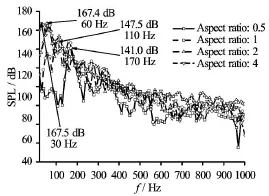
Fig.8 The flow-induced noise frequency spectrum of four different aspect ratio models

Because the acoustic wavelength exceeds any characteristic dimension of the cavity， the coupling effect between the hydrodynamic field and the sound field can be ignored. The hole surface shapes and the aspect ratios are the main factors that influence the contribution of the sound source at the tail edge. From Eq.（9）， the flow direction scale of the hole mouths dominates the fundamental frequencies. Therefore， with the increase of the flow direction scale （length） of the hole mouths， the fundamental frequencies move to the low frequency region with an increased level of the radiation noise. Whereas， with the increase of the flow vertical direction scale （width） of the hole mouths， the scale and the strength of the sound source increase linearly. In view of the effect of this two direction scales， under the conditions of the same area， in the case of the aspect ratios close to 1， the flow-induced noise level of the open cavity will be reduced. It is easily understood that the flow-induced noise of the circle or square shape models has much low level than others.

Table 4 The sound power level of six different hole neck angle models

3.4 Effects of hole neck angles

In order to study the effects of the hole neck angles on the flow-induced noise， a series of the hole neck angle models are established in Table 4. Because the other flow conditions and structure parameters remain unchanged， the hydroacoustics data of the boundary layer of these models are almost the same. However，in view of the impingement of the vortical perturbations on the downstream corner， the effects of the hole neck angles will be important and must be considered.

Fig.9 The flow-induced noise frequency spectrum of six different hole neck angle models

From Fig.9， it is clearly observed that the frequency spectrum configuration sees a significant alteration due to the change of the angle. In these curves，the spectral profiles of the 30omodel and the 45omodel have no obvious peak. It can be explained by the impingement at the downstream cavity edge where the downstream cavity edges of the 30omodel and the 45omodel have a similar tangent of the vortex rotation. The flow impact energy is small， so the self sustained oscillation will be weak. Thus， the flow-induced noise level will be effectively reduced. As the hole neck angle reduces， the amplitude of the fundamental frequency decreases. However， when the angle is smaller than a certain constant value， the amplitude of the low frequencies increases and determines the radiated noise level. In Table 4， the OSPL of the 45omodel is approximately 115.9 dB， less than that of the 90omodel: 150.9 dB. In view of the reduction， the hole neck angle is one of the most effective parameters for the low-noise design.

Table 5 The sound power level of four different horizontal porous models （“2 of 4” means the second hole of the four hole model along the flow direction）

Table 6 The sound power level of four different vertical porous models （“2 of 4” means the second hole of the four hole model from the symmetry centre to side wall）

3.5 The horizontal and vertical porous cases

Actually， the underwater structure cavities usually involve not only a single hole design. In order to study the effects of porous arrangements on the flowinduced noise， the horizontal and vertical porous casesare considered by a series of porous models （i.e.， 1， 2，4， 8 holes）. The CFD and the acoustic field computation boundary remain the same as the original model. The scale of the holes is also as defined in Fig.1，where α=90oand the distance between the two adjacent holes is 5 mm. A hydrophone is located in the center of each hole.

The OSPLs of the radiated noise are calculated for the horizontal porous and vertical porous models as shown in Table 5 and Table 6. The OSPL of the horizontal porous models （i.e.， 2， 4 holes） is approximately 10 dB more than that of the vertical porous models， while the OSPLs of two models with 8 holes are much closer to each other. In the same horizontal porous model， the radiated noises at the measurement points are close to each other except the last hole along the flow direction， at which a much higher level of the radiated noise is found. Meanwhile， in the same vertical porous model， the levels of the radiation noises at the measurement points from the symmetrical centre to the side wall are reduced gradually.

Fig.10 The flow-induced noise frequency spectrum of four horizontal porous models

Fig.11 The flow-induced noise frequency spectrum of four vertical porous models

From the frequency spectrum configurations of the horizontal porous models shown in Fig.10， it is indicated that as the number of holes increases， the amplitudes of the low frequencies below the fundamental frequency increase and the signal to noise ratios of the fundamental frequency decrease. It is mainly caused by the flow interaction between the holes and the cavity， by which the large eddy energy of low frequency can be enhanced by increasing the number of holes. However， from Fig.11， it is seen that as the number of holes increases， the amplitudes of the fundamental frequency become higher and higher than the other frequencies. It means that the flow interaction between the holes can be ignored and the acoustic field can be calculated by the principle of superposition， but just for the same vertical porous model.

Fig.12 The flow field of the 18 horizontal porous model （a section of the hole mouth）

3.6 Effects of incoming flow attack angle by using a submarine horizontal porous model with 18 holes

In an underwater structure cavity such as the tail of a submarine， we must consider the angles between the incoming flow direction and the open cavity mouth surface. In this part， the effects of the flow attack angle on the flow-induced noise are discussed. According to the actual scale of a horizontal porous submarine cabin， the model of the open cavity with 18 holes is established as shown in Fig.12. A hydrophone is placed in the center of the middle hole. The open cavity hydroacoustics data of the three flow attack angle cases are shown in Table 7.

From Table 7 and Fig.13， three models （i.e.，0o，5o，45oattack angle modes） are chosen for the CFD and acoustic computations. It is remarkable to see that the attack angle parameter influences not only the OSPL of the acoustic radiation but also the tone frequency significantly. The fundamental frequency of the0°model is 21.6 Hz， much close to 21.4 Hz obtained by equation 8. When the attack angle is changed slightly to 5°， the fundamental frequency becomes 16 Hz， and the amplitude of the peek frequency decreases from a value of approximately 149.7 dB to 141.6 dB. But when the attack angle increases to45o，there is no tone frequency but with higher level of flow-induced radiated noise.

This numerical analysis of the actual submarine open cavity models reveals some interesting results. First， in the horizontal porous model with 18 holes，the semi-empirical formula （Eq.（9）） for the classical rectangular cavity is still valid. Second， a low attackangle can change the flow-induced noise frequency spectrum significantly. Because， as the attack angle increases， the vortex shedding speed at the leading edge reduces and the eddy scale increases. Thus， the tone frequency shifts to the low frequency region. This result is worth more attention for the second noise radiation by the flow-induced structure vibration when the flow-induced tone frequency is close to the natural frequency of the underwater structure.

Table 7 The open cavity hydroacoustics data of different boundary layer thickness models

Fig.13 The flow-induced noise frequency spectrum of three attack angle models

4. Conclusions

Based on the FW-H acoustic analogy， the flowinduced noise of the underwater structure cavities is discussed. In order to study the self-sustained oscillations of the cavity flow and the mechanisms of the cavity noise generation， a series of three-dimensional open cavity models are established based on the simplified model. Several important conclusions are drawn from the analysis:

（1） In the case of a low Mach number water flow，the radiated noise is dominated by the dipole source of the FW-H equation， whereas the monopole source and the quadrupoles source can be neglected. The splitting method to turn the hydroacoustics analysis into the analysis of an incompressible flow and the acoustic analysis is effective and convenient for the numerical calculation.

（2） With the increase of the flow speed， a higher level of noise is radiated to the sound field from the open cavity， and the fundamental frequency remains almost the same as that determined by using the Strouhal number equation.

（3） As the boundary layer thickness increases， the tonal frequency and the OSPL decrease slightly. However， the largest amplitude of the tonal components is found in the case of an intermediate boundary layer thickness.

（4） The circle or square shape of the cavity mouth and the aspect ratios close to 1 will reduce the flow-induced noise level of the open cavity.

（5） The neck angles of the hole affect the noise level greatly. The OSPL of the 45omodel is approximately 34 dB less than that of the90omodel. In view of the reduction， the hole neck angle is one of the most effective parameters for a low-noise design.

（6） In the horizontal and vertical porous cases，the semi-empirical formula （Eq.（6）） for the classical rectangular cavity is still valid. In the horizontal porous models， the flow interaction between the holes and the cavity can enhance the large eddy energy of low frequency， whereas it can be ignored in the vertical porous models.

（7） For the actual submarine open cavity model with an incoming flow attack angle of5o， the fundamental frequency turns to 16 Hz from 21.6 Hz， and the amplitude of the peak frequency is decreased from a value of approximately 149.7 dB to 141.6 dB.

References

［1］ GLOERFELT X.， BAILLY C. and JUVÉ D. Direct computation of the noise radiated by a subsonic cavity flow and application of integral methods［J］. Journal of Sound and Vibration， 2003， 266（1）: 119-146.

［2］ ASHCROFT G. B.， TAKEDA K. and ZHANG X. A numerical investigation of the noise radiated by a turbulent flow over a cavity［J］. Journal of Sound and Vibration， 2002， 265（1）: 43-60.

［3］ JIN Y.， UTH M. F. and HERWIG H. Structure of a turbulent flow through plane channels with smooth and rough walls: An analysis based on high resolution DNS results［J］. Journal of Computers and Fluids， 2015，107: 77-88

［4］ SANDBERG R. D. Direct numerical simulations for flow and noise studies［J］. Procedia Engineering， 2013，61: 356-362.

［5］ HILEWAERE J.， DOOMS D. and QUEKELBE-RGHE B. V. et al. Unsteady Reynolds averaged Navier-Stokes simulation of the post-critical flow around a closely spaced group of silos［J］. Journal of Fluids and Stru-ctures， 2012， 30: 51-72.

［6］ LIU Zheng-gang， DU Guang-sheng and LIU Li-ping. The analysis of flow characteristics in multi-channel heat meter based on fluid structure model［J］. Journal of Hydrodynamics， 2015， 27（4）: 624-632.

［7］ GLOERFELT X. Large-eddy simulation of a high Reynolds number flow over a cavity including radiated noise［C］. The 10th AIAA （American Institute of Aeronautics and Astronautics）/CEAS Aeroacoustics Conference. Manchester， UK， 2004.

［8］ CHEN Shi-yi， CHEN Ying-chun and XIA Zhen-hua et al. Constrained large-eddy simulation and detached eddy simulation of flow past a commercial aircraft at 14 degrees angle of attack［J］. Science China Physics， Mechanics and Astronomy， 2013， 56（2）: 270-276.

［9］ CASALINO D. An advanced time approach for acoustic analogy predictions［J］. Journal of Sound and Vibration， 2003， 261（4）: 583-612.

［10］ ASK J.， DAVIDSON L. An acoustic analogy applied to the laminar upstream flow over an open 2D cavity［J］. Comptes Rendus Mecanique， 2005， 333（9）: 660-665

［11］ SPALART P. R. On the precise implications of acoustic analogies for aerodynamic noise at low Mach numbers［J］. Journal of Sound and Vibration， 2013， 332（11）: 2808-2815.

［12］ WANG Yu， WANG Shu-xin. Influence of cavity shape on hydrodynamic noise by a hybrid LES-FW-H method［J］. China Ocean Engineering， 2011， 25（3）: 381-394.

［13］ ZHANG Nan， SHEN Hong-cui and YAO Hui-zhi. Numerical simulation of cavity flow induced noise by LES and FW-H acoustic analogy［J］. Journal of Hydrodynamics， 2010， 22（5）: 242-247

［14］ ZHANG Y. O.， ZHANG T. and OUYANG H. et al. Flow-induced noise analysis for 3D trash rack based on LES/Lighthill hybrid method［J］. Journal of Applied Acoustics， 2014， 79（3）: 141-152.

［15］ GENG Dong-han， WANG Yu. Prediction of hydrodynamic noise of open cavity flow［J］. Transactions Tianjin University， 2009， 15（5）: 336-342.

［16］ YOO S. P.， LEE D. Y. Time-delayed phase-control for suppression of the flow-induced noise from an open cavity［J］. Applied Acoustics， 2008， 69（3）: 215-224.

［17］ SUN J.， YANG G. and LIANG Y. et al. Expermental study of boundary layer effect on the aeroacoustic characteristics of the incompressible open cavity［J］. AASRI Procedia， 2014， 9: 44-50

［18］ BOGEY C.， BAILLY C. Large eddy simulations of round free jets using explicit filtering with/without dynamic Smagorinsky model［J］. International Journal of Heat and Fluid Flow， 2006， 27（4）: 603-610.

10.1016/S1001-6058（15）60529-7

（October 26， 2013， Revised August 18， 2014）

* Biography: YUAN Guo-qing （1984-）， Male， Ph. D.

JIANG Wei-kang，

E-mail: wkjiang@sjtu.edu.cn