
Mechanical Behavior of Flexible Jumper Installation in 3D Space
2015-12-12 08:52LIUTingRUANWeidongSHIYouFUJianboYANGHonggang
船舶力学 2015年6期
LIU Ting,RUAN Wei-dong,SHI You,FU Jian-bo,YANG Hong-gang
(1 Department of Civil Engineering,Zhejiang University,Hangzhou 310058,China;2 Offshore Oil Engineering Co.,Ltd,Tianjin 300451,China;3 CNPC Baoji Oilfield Machinery Co.,Ltd,Baoji,721002,China)
0 Introduction
In subsea oil/gas production systems,subsea jumpers are short pipe connectors used to transport production fluids between two subsea components;for example,tree and manifold,manifold and manifold,or manifold and export sled[1].Within the past decades the application of jumpers in subsea structures has increased greatly.Among the applications,the flexible jumper stands out due to its strong compliant characters,excellent fatigue design life,and high resistance to collapse,etc.However,the actual installation process of the flexible jumper requires special attention,as when it is lowered into deep water by cables,the configuration of the flexible jumper depends highly on the applied load(the environment factors)and the installation methods used.Therefore,the flexible jumper is easily capable of reaching its minimum allowable bend radius and its limited axial tension.In order to guarantee the accuracy and security of the flexible jumper’s installation,the displacement of the whole system,includ-ing the jumper and cables in a 3D space,should be carefully discussed and the axial tension should also be accounted for.
Recently,many advances have been made in the area of study relating to flexible jumpers.Huang et al[2]has previously done research on flexible jumper VIV under a uniform current;its motion was predicted through a simplified catenary riser motion solver that superposes a static catenary solution with a tensioned beam’s motion equation;the results showed the simulation worked well when applying this kind of theory.However,the actual subsea condition is quite complicated,the direction and velocity of the current can change significantly in different water depths.Fernandes et al[3]identified the critical issues and devised a design procedure that addressed the highly compliant riser system,in which the two connection points were positioned at the same level.Huang et al[4]presented analytical and numerical approaches for the optimum design and global analysis of flexible jumpers on the basis of Fernandes et al.Huang et al[4]also developed the critical length for the optimum design,in which,the two connection points were positioned at different levels.The above two literatures on the analysis of flexible jumpers are essentially limited to two-dimensional or planer loadings and deformations,and cannot be used to accurately describe the shape of 3D flexible jumpers.Chai et al[5]put forward an absolute coordinate formulation for three-dimensional flexible pipe analysis by expressing the structural response characteristics in terms of globally based position coordinate and its derivative.This allows for a non-linear description of the pipe kinematics to be made.Ahmadizadeh[6]proposed an iterative method for three-dimensional large-displacement analysis of structures,which consists of slack cables that act as a primary load-bearing system.Although Ahmadizadeh’s study mainly focused on the analysis of simply suspended cables that have considerable amounts of sag,his proposed methods used to address the space structureslack cables,were used within this specific research when dealing with the installation of flexible jumpers.
In this paper,an iterative procedure is presented regarding the installation process of a flexible jumper that is lowered into deep water by cables in a 3D space.The initial form(only subjected to dead gravity loads along the entire length)of the installation system can be obtained using the catenary theory.The main purposes of this procedure are:determine the original environmental loads applied to each of the different segments of the cables and the flexible jumper in various water depths;approximately define,under environmental loads,the starting point’s reaction that will be used in the iterative procedure to reform the system.The configuration,internal force and the bend radius of the flexible jumper can be calculated after the system satisfies the compatibility and equilibrium requirements.In order to verify the accuracy and reliability of the proposed method,an illustrative analysis example is carried out and the results are compared with those derived from an OrcaFlex finite-element model.The influence on the minimum bend radius and maximum axial tension of the flexible jumper due to the difference between the lowering cable lengths on both sides,is also studied.
1 Configuration of the installation system
A schematic of the process used to install flexible jumpers in practical engineering can be seen in Fig.1.
For the sake of convenience,the installation model can be simplified for the analysis,and the following assumptions can be made:
(1)During the installation process,the positions of the two top points of the cables remain unchanged.

Fig.1 Flexible jumper installation
(2)The bending stiffness of the flexible jumper can be negligible,as it will not have a significant effect on the kinematics.
(3)Compared to the length of the cables and the flexible jumper,the length of the bend restrictor,gooseneck,connector actuation tools(CATs)and the other accessories are actually quite short.Thus,they can be treated as a singular element;the equivalent length,weight and diameter can be used to describe this element,whose antonomasia will be bend restrictor in the following sections of this paper.
1.1 The initial configuration of the system
In order to create a starting point for the iterative procedure,an initial trail form needs to be chosen.For simplicity,a two-dimensional shape in the XZ plane is chosen as the initial form,and Point A is selected as the starting point,as illustrated in Fig.2.The cables and the flexible jumper meet catenary conditions,and the flexible jumper can be divided into two parts at its lowest point,M,thus,there are four catenary segments in total.

Fig.3 3D mechanics analysis model of flexible jumper installation
According to the catenary theory,the following equations can be obtained.
The projection lengths of Segments AE and BF on the Z axis Hwir-AE,Hwir-FBand X axis Swir-AE,Swir-FBare presented below,respectively:


where a is the characteristic length of the flexible jumper,defined by the ratio of the horizontal component THand wjum.wjumand wwirare the distributed weight of the flexible jumper and the cables,respectively.
The vertical projections of Segments IM and MJ of the flexible jumper,Hjum-IMand Hjum-MJ,can be expressed by the corresponding horizontal projections Sjum-IMand Sjum-MJ,
The total length of the flexible jumper Ljumcan be expressed as

And the vertical compoents of Points A,B E,F can be evaluated as:
where GEand GFrepresent the equivalent weight of the bend restrictor elements EI and FJ.
According to the equilibrium of the bending moment and the geometric relationship of the bend restrictor element in Points E and F,the following equations are obtained.
where SE,HE,SFand HFare the vertical and the horizontal projections of element EI and FJ.
Besides,the system should also satisfy the compatibility requirements;that is,
where SABrepresents the horizontal distance from Point A to Point B in the XZ plane,and HABis the vertical distance between the two end points.
When the cables and flexible jumper are surbmerged in water,the bouyant force should be subtracted from the dry weight.The 17 unknowns in the 17 equations can be solved simultaneously.The intial form of the installation system can then be obtained.In order to reduce the iterations needed to determine the final shape,the environmental loads in the X and Y axis directions,for the left half of the system(seperated at the lowest point,M),are added to the corresponding components presented at the starting point,A.
1.2 Form and internal force of the system under environmental load
The initial catenary form,assumed for the installation system,is not in equilibrium and does not satisfy the compatibility requirements under environmental loads.Thus,an iterative procedure needs to be adopted,as to update the system form and internal forces,in order to satisfy those requirements.
As illustrated in Fig.3,a 3D coordinate system is set up by first locating the origin at the position of Point A;the origin of the local frame of reference is then set at node i-1.The flexible jumper and cables can be divided into short straight elements,and the bend restrictor can be regarded as a single element.Therefore,in total,there areelements.The number of flexible jumper divisions nEFand cables divisions nAE,nBFcan be selected based on the required precision and the processing cost.Assuming that,the X-axis direction is in parallel with the wave direction,the water particle velocity u and water particle acceleration du/dt caused by waves can be derived based on Airy’s theory.

where Hsis the wave height,Tsis the wave period,λ is the wave length,DWis the water depth,and HACis the vertical distance from Point A to the sea surface.
Based on the Morison formula and geometric relationship,the horizontal force acting on each element in the x-axis and y-axis directions can be expressed as,
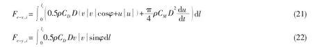
where ρ is the density of water,CDis the drag coefficient,CMis the inertia coefficient,D is the outer diameter of the element,v is the current velocity,and φ is the current direction.liis the length of the ith element,its value should be taken accordingly from the corresponding divisions of each part.
The initial assumption of the starting point’s reaction in the iterative procedure(TX,0,TY,0,TZ,0)1can be obtained from the method presented previously in Part 1.1;the subsequent nodal forces can be derived as follows:

where the subscript i is the element number,TX,i,TY,i,TZ,iare the nodal component forces,and Giis the element weight.When the element is submerged in water,the buoyancy force should be subtracted.
The bending stiffness of the cable and flexible jumper can be neglected.Therefore,Element i lies along the direction of the resultant force Ti,and the new location of the pointcan be determined using the following equation:

When the locations of the subsequent points are all updated,the last node(the other supporting Point B’s position)can be obtained.However,Point B’s position derived from the procedure presented above does not necessarily coincide with the actual point.Thus,the assumed starting point’s reaction should be modified and the next iteration calculating the point locations begins until the relative error in the prediction of point B is small enough;the adjustment of the initial force can be decided based on the below guidelines:

where SAB,YAB,HABare the actual horizontal distances along the X-axis,Y-axis and the vertical distance along the Z-axis from Point A to Point B;γ is the proportional gain which controls the magnitude of the correction made on the starting point’s components;usually,it is chosen to equal 0.001,or smaller if the analysis does not converge.The subscript n represents the iterative number.If the difference in the values of the derived ones and the actual ones is negative,then the corrections should be made in the adverse directions,that is to say,if ZB-then,should decrease;the sign of operator should change to its adverse one:It is the same with the other two components.This procedure is repeated until the calculated relative error of Point B is less than a certain specified value,and ε is the predetermined convergence tolerance.

After determining the exact position of each node in the system,the axial force of the node along the cables and the flexible jumper can be derived as:

During the installation,the bend radius of the flexible jumper must be taken into consideration,as it can easily reach the limited minimum bend radius,bringing on many potential detriments.Therefore,the bend radius needs to be calculated in order to check whether it is safe or not;it can be obtained using the following equation,

where:

2 Finite-element analysis(FEA)modeling
The installation of the flexible jumper can be simulated using the commercial software OrcaFlex[7].The schematic of the OrcaFlex model can be seen in Fig.4.A line type is used to simulate the flexible jumper and the lowering cables,and the two top ends are pin joints.

Fig.4 Sketch of OrcaFlex model
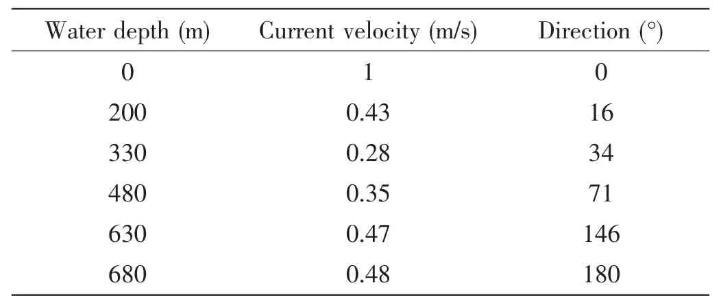
Tab.1 Data for current profile

Tab.2 Parameters of sea water and wave
In the FEM,current is assumed to be steady;its direction is set as 0°when it is in parallel with the X-axis,and 180°when in the reverse direction.The current velocity and the direction in various water depths can be derived through the interpolation method,while the wave type is adopted from the single Airy model.The parameters of the current can be seen in Tab.1,and the other environment,flexible jumper,lowering cables and bend restrictor data are listed in Tabs.2-5.

Tab.3 Parameters of the cable
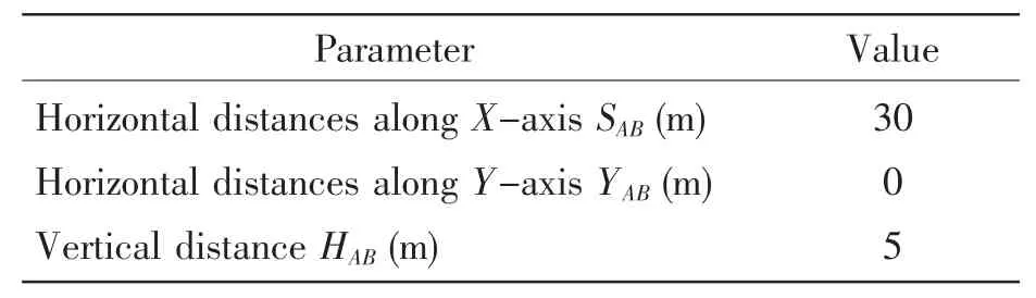
Tab.4 Geometrical relationship of Points A and B
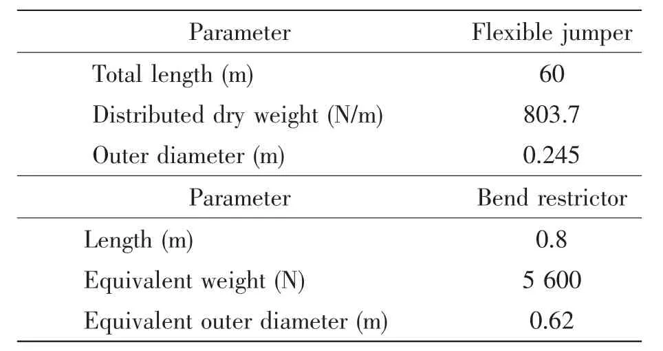
Tab.5 Parameters of flexible jumper and bend restrictor
3 Comparison and discussion
In order to verify the accuracy and reliability of the method presented above,comparisons are carried out between the results obtained from the OrcaFlex simulation and from the proposed method.
Fig.5 shows the comparison of the axial tension along the length of the system.The results derived from the proposed method are similar to those achieved from the OrcaFlex simulation,and the differences between the two solutions are less than 5%.The axial tension of the flexible jumper along its length can be seen clearly in Fig.6.It can be observed that the minimum axial tension occurs at the lowest point of the flexible jumper,and increases along the length of the flexible jumper in both the left and right directions.The difference in the axial tension in the two tail ends of the flexible jumper is closely related to the difference in the length of the lowering cables on the two sides.
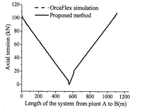
Fig.5 Comparison of the axial tension along the length
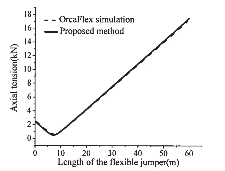
Fig.6 Comparison of the axial tension of flexible jumper
The three dimensional displacement curves of the installation system derived from the proposed method and the OrcaFlex simulation are shown in Fig.7.From the curves,it can be noticed that,the displacement in the YZ plane are in good agreement with each other.However,there exists a certain deviation in the XZ plane,especially in the section to the right of the installation system.This is so because of the accumulation of the displacement difference from the starting point to the corresponding point in the curve;the element number of the system may also contribute to the difference in the displacement.However,the general trend of the displacement is substantially uniform.Thus,this proposed method can give a good estimation of the mechanical behavior of the flexible jumper installation system.
A comparison of the bend radius along the length of the flexible jumper from the two solutions is presented in Fig.8.The graph indicates that,the minimum bend radius also appears at the lowest point of the flexible jumper.Thus,this point requires special attention during the installation process.Though,the results obtained from the OrcaFlex simulation just roughly agree with the ones achieved from the proposed method,the minimum bend radius for both seem to be in good agreement,which is the core concern of the engineer.The results can also give some reference to practical engineering of estimating the minimum bend radius.

Fig.7 Comparison of the displacement in 3D space

Fig.8 Comparison of the bend radius of flexible jumper

Fig.9 Axial tension of flexible jumper with different lengths of Cable BF

Fig.10 Bend radius of flexible jumper with different lengths of Cable BF
Fig.9 and Fig.10 show the axial tension and the bend radius along the length of the flexible jumper with different lengths of Cable BF.With the increase of the length of the Cable BF,the difference in the level between the two end points of the flexible jumper decreases.Therefore,the maximum axial tension along the flexible jumper becomes smaller.If the length of Cable BF exceeds the length of Cable AE,the maximum axial tension will gradually be aggrandized;this characteristic can be seen more explicitly in Fig.11,where the height difference between Points A and B has been taken out.It is obvious that,in order to decrease the maximum axial tension of the flexible jumper,it is better to keep the two end sides of the flexible jumper at the same level.
It seems that,the altitude difference of the two end points of the flexible jumper has little impact on its minimum bend radius when compared with the variations of the maximum bend radius,seen in Fig.10.The OrcaFlex simulation results show that:when the two end points of the flexible jumper are in the same level,the minimum bend radius is 2.258 m and the maximum is 459.94 m;when the altitude difference is 45 m,the minimum bend radius is 2.091 m and the maximum is 997.96 m.Though,there is not much difference in the numerical values of the minimum bend radius it may still make a difference in the safety of the flexible jumper during installation.

Fig.11 The relationship of maximum axial tension with the altitude difference of the two end points
4 Conclusion
In this paper,the installation of a flexible jumper lowered into deep water by cables is studied in a 3D space,and the results obtained from the theoretical analysis are compared with the ones achieved from the OrcaFlex simulation.The two sets of results are in good agreement,and it can be concluded that:
Though,the minimum axial tension of the flexible jumper occurs at the lowest point along its length during the installation,the minimum bend radius also occurs at this point.Thus,this point becomes very dangerous during the installation process and requires special attention.In order to reduce the maximum axial tension of the flexible jumper,it is better to keep its two end points in the same level by making both the lowered cable lengths equal on the two sides.The displacement of the installation system,especially the two end points of the flexible jumper,which connect the joint devices,can be estimated and a more appropriate parting position in the sea surface of the installation vessel can be chosen on the basis of this estimated value.
[1]Bai Yong,Bai Qiang.Subsea engineering handbook[M].USA:Gulf Professional Publishing,2010:664.
[2]Huang Kevin,Chen Hamn-Ching.Flexible jumper VIV simulation in uniform current[C]//Proceedings of the Twenty-first International Offshore and Polar Engineering Conference,June 19-24,2011.Maui,Hawaii,USA,2011:1297-1304.
[3]Fernandes A C,Silva R M C,Carvalho R A,Lemos C A D,Jacob B P.Alternative design of flexible jumpers for deepwater hybrid riser configurations[J].Offshore Mech.Arct.Eng,2001,123(2):57-64.
[4]Huang Yi,Zhen Xingwei,Zhang Qi,Wang Wenhua.Optimum design and global analysis of flexible jumper for an innovative subsurface production system in ultra-deep water[J].China Ocean Engineering,2014,28(2):239-247.
[5]Chai Y T,Varyani K S.An absolute coordinate formulation for three-dimensional flexible pipe analysis[J].Ocean Engineering,2006,33:23-58.
[6]Ahmadizadeh M.Three-dimensional geometrically nonlinear analysis of slack cable structures[J].Computers and Structures,2013,128:160-169.
[7]Orcina,2009.OrcaFlex Manual,Version 9.3a[K].UK.

- 船舶力学的其它文章
- DES Simulation of Flow Field of Propeller Tip Vortex
- Numerical Study on the Hydrodynamic Behaviors of a Ship Passing Through a Lock in Shallow Water
- Characteristics of Tendon Vortex Induced Vibrations Influenced by Platform Motion
- Load-Compression Relationship of Incompressible Circular Rubber Pad Bonded between Rigid Plates
- Two-dimensional Eulerian-Lagrangian Modeling of Shocks on an Electronic Package Embedded in a Projectile with Ultra-high Acceleration
- Influence of Excitation Location on Sound Radiation of a Simple Duct Excited by Sound Source