Numerical study of roll motion of a 2-D floating structure in viscous flow*

Lifen CHEN， Liang SUN， Jun ZANG， A. J. HILLIS， A. R. PLUMMER

1. WEIR Research Unit， Department of Architecture and Civil Engineering， University of Bath， Bath， UK，

E-mail:chenlifen239@gmail.com

2. Department of Mechanical Engineering， University of Bath， Bath， UK



Numerical study of roll motion of a 2-D floating structure in viscous flow*

Lifen CHEN1， Liang SUN1， Jun ZANG1， A. J. HILLIS2， A. R. PLUMMER2

1. WEIR Research Unit， Department of Architecture and Civil Engineering， University of Bath， Bath， UK，

E-mail:chenlifen239@gmail.com

2. Department of Mechanical Engineering， University of Bath， Bath， UK

In the present study， an open source CFD tool， OpenFOAM has been extended and applied to investigate roll motion of a 2-D rectangular barge induced by nonlinear regular waves in viscous flow. Comparisons of the present OpenFOAM results with published potential-flow solutions and experimental data have indicated that the newly extended OpenFOAM model is very capable of accurate modelling of wave interaction with freely rolling structures. The wave-induced roll motions， hydrodynamic forces on the barge， velocities and vorticity fields in the vicinity of the structure in the presence of waves have been investigated to reveal the real physics involved in the wave induced roll motion of a 2-D floating structure. Parametric analysis has been carried out to examine the effect of structure dimension and body draft on the roll motion.

OpenFOAM， CFD， potential-flow theory， roll motion， 2-D floating structure， regular waves， wave forces， viscous flow

Introduction

The hydrodynamic motions of ships and floating structures in the presence of waves need to be carefully examined during the early stage of structure design to ensure the stability characteristics or energy efficiency of the structure. In reality， a ship or floating structure experiences motion in all six degrees of freedom （DoF） simultaneously， but only roll motion will be investigated in this paper. Roll motion is the most critical motion leading to ship or platform capsizes compared to other five degrees of freedom motion of a ship or platform［1，2］. The roll motion of a ship or floating structure can be determined by solving an ordinary differential equation which contains three coefficients， the virtual mass moment of inertia for rolling， the damping coefficient and the restoring moment coefficient. The value of these three coefficients can be determined experimentally or by using mathematical methods. Among them， the damping coefficient has been considered to play the most significant role in the roll motion calculation and should be determined accurately. Model test has been one of the most common approaches used to estimate the roll damping. Generally， the body is rolled to a chosen angle and then released in calm water. The recorded roll time history is used to determine the equivalent linearized roll damping by assuming that the dissipated energy due to the nonlinear and equivalent linear damping is the same. Jung et al.［3］carried out several experiments in a 2-D wave tank to study the roll motion of a rectangular barge and concluded that the roll damping in some wave conditions helps the barge to roll. Wu et al.［4］conducted an experimental investigation to study the nonlinear roll damping of a ship in the presence of both regular and irregular waves. The recorded roll time history in calm water obtained by Wu et al.［4］had the similar trend with that obtained by Jung et al.［3］.

Physical experimentation is expensive and not always practical. Numerical methods， including potential flow theory， empirical formula and viscous flow theory， have also been widely used for the prediction of the roll motion. Potential flow theory like strip theory is applied to investigate wave induced roll motion based on the assumption that the motion of a floating structure by waves is linear. Lee et al.［5］used strip theory to investigate the roll damping of a ship in beam seas and the hydrodynamic radiation damping ofa rectangular barge， respectively. The potential flow theory has been used to predict the motion of the structure in surge， heave， pitch， sway and yaw to a reasonable degree of accuracy without any empirical correction or recourse to experiments. However， it is found that the wave damping derived from the linear potential flow theory is inadequate for an accurate prediction of the roll motion since the effect of viscous damping could be as significant as those of wave damping in roll［6］.

One of the compensating methods is to introduce an artificial or empirical damping coefficient in the computation using potential flow theory to take into account the viscous effect. Chakrabarti［6］divided the total roll damping coefficient into several components，such as friction， eddy， wave damping， lift etc.. Wave damping is derived from linear potential flow theory while other components can be computed by empirical formulas. This prediction method has been applied successfully by inviscid-fluid models coupling with the strip theory［7］.

The applicability of the empirical formulas is limited by the fact that the empirical coefficients are derived from extensive model tests or field measurements. Viscous models based on Navier-Stokes equations are becoming increasingly popular in engineering predictions for providing more accurate and realistic results. Zhao and Hu［8］developed a viscous flow solver， based on a constrained interpolation profile（CIP）-based Cartesian grid method， to model nonlinear interactions between extreme waves and a boxshaped floating structure， which is allowed to heave and roll only. Bangun et al.［9］calculated hydrodynamic forces on a rolling barge with bilge keels by solving Navier-Stokes equations based on a finite volume method in a moving unstructured grid. The roll decay motion of a surface combatant was predicted by Wilson et al.［10］using an unsteady Reynoldsaveraged Navier-Stokes （RANS） method. The RANS method was employed by Chen et al.［11］as well to describe large amplitude ship roll motions and barge capsizing.

OpenFOAM， an open-source CFD package， is proved to provide accurate numerical predictions when applied to nonlinear wave interactions with fixed structures. Morgan et al.［12，13］has extended the OpenFOAM and reproduced the experiments on regular waves propagation over a submerged bar successfully with up to 8th order harmonics correctly modelled. The extended OpenFOAM has been applied to model nonlinear wave interactions with a vertical surface piercing cylinder and a single truncated circular column by Chen et al.［14］and Sun et al.［15］， respectively. The accuracy of the models was validated by comparing with experiments. A built-in dynamic solver interDyMFoam was extended by Ekedahl［16］to simulate wave-induced motions of a floating structure.

The model diverged after about 10 s for the case with a coarse mesh due to numerical discrepancies or low mesh quality. According to Yousefi et al.［17］，OpenFOAM can also be applied to simulate the flow field around a hull， taking into account maneuverability， wave and free surface effects and it is gaining increasing popularity due to its excellent computational stability.

In this paper， the nonlinear interactions between regular waves and a 2-D rolling rectangular barge have been studied numerically and the results are compared with the experimental measurements collected by Jung et al.［3］. The extended OpenFOAM model developed by Chen et al.［14］is selected here for the two-phase flow modeling as well as wave generation and absorption. Two difficulties have been solved in order to extend its capability of simulating the roll motion of floating structures by waves: determining the wave-induced motion of the floating structure and moving or deforming the mesh according to this motion. The wave-induced roll motions， hydrodynamic forces on the barge， velocities and vorticity flow fields in the vicinity of the structure in the presence of waves have been investigated in this paper. Parametric analysis has been carried out to study the effect of the structure size and draft on the roll motion.

1. Numerical methods

1.1 Flow Fields

The extended OpenFOAM model developed by Chen et al.［14］has been selected here for the two-phase flow modelling based on the unsteady， incompressible Navier-Stokes equations. The waves are generated by introducing a flux into the computational domain through a vertical wall and the wave reflections at the end of the wave flume are dissipated by a numerical beach in the extended OpenFOAM model.

1.1.1 Governing equations

The flow fields are solved using the laminar form of the Navier-Stokes equations for an incompressible fluid as follows:

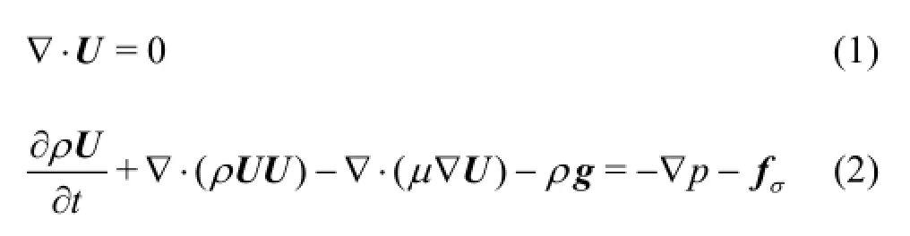
in whichU is the fluid velocity，pis the fluid pressure andfσis the surface tension.ρandµare the fluid density and the dynamic viscosity， respectively.

The free surface is tracked by using the volume of fluid （VOF） method and indicated by the volumefraction functionαwhich ranges from 0 to 1， where 0 and 1 represent air and water， respectively. The volume fraction function can be calculated by the following equation

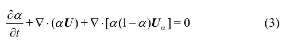
where the last term on the left-hand side is an artificial compression term used to limit numerical diffusion and Uαis the relative compression velocity［18］.

1.1.2 Boundary conditions

（1） Wave inlet boundary conditions

The volume fraction functionαand the velocities are specified on the inlet boundary.αis determined based on the location of the face centre relative to the free surface elevation η（x， z， t）and can be calculated by a simple limiting function

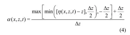
where ∆zis a small parameter specifying the width of the water-air interface. In the VOF technique， the boundary is assumed to be a straight line that cut through the cell containing the free surface. The width of this thin line is assigned to be∆zhere which can be pre-defined by the users. The velocities on the inlet boundary are calculated by multiplying the velocities from the selected wave theory byαso that the velocities in the air are zero and the velocities in the water are as calculated.

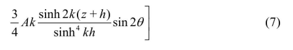
In this study， 2nd order Stokes' wave theory for arbitrary depth is used in which，θ=kx-ωtandk is wave number，ω is angular velocity andA is wave amplitude.

（2） Far field boundary conditions

In this study， a numerical beach is used to minimize the wave reflection at the downstream of the flume by damping the momentum energy. An artificial damping term，ρθU ， is added to the momentum equation， and then Eq.（2） can be rewritten as［14］

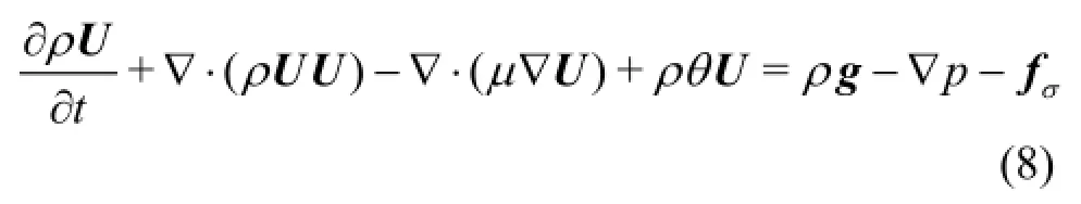
in which

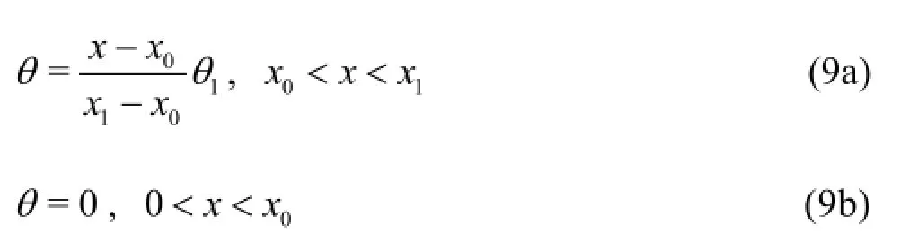
wherex is the coordinate from wave generator，x0is the start point of the damping zone，（x1-x0）is the length of the damping zone and θ1is the damping coefficient. There is little dissipation by using small damping coefficients while for large values of damping coefficient the damping zone itself will act as a boundary and wave reflection occurs at the beginning of the relaxation zone. The length of the damping zone and the value of the damping coefficient are determined empirically and numerical tests are carried out if necessary. Details on the performance and validation of this method are given by Chen et al.［14］.

1.2 Wave-induced roll motion of a floating structure

New modules have been developed based on interDyMFoam， a built-in OpenFOAM viscous-solver for multiphase problems with moving boundaries， to extend its capabilities to simulate the roll motion of floating bodies in the presence of waves. Two difficulties have been solved: determining the location of the floating structure and updating the mesh automatically according to the motion of the structure.

1.2.1 The equation of roll motion

The roll motion of a moving object can be determined by solving the equation of motion

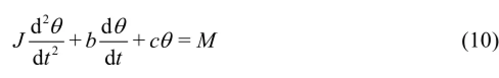
where Jd2θ/dt2is the inertial moment in whichJrepresents the mass moment of the inertia and d2θ/dt2is the angular acceleration.bdθ/dtis the damping moment in whichbis the damping moment coefficient and dθ/dtis the angular velocity.cθis the restoring moment in whichcis the restoring moment coefficient andθis the angular displacement of rotation.M is the external angular torque which can be calculated by summing the moments about the COG over the body due to the pressure forces obtained by solving Eq.（1） and Eq.（8）. Similar to De Bruijn et al.［19］only pressure forces were considered， since viscous forces are negligible in this wave application when laminar flow solver was used in the model. The angular velocity dθ/dtabout the COG can be obtained by solving the motion equations Eq.（10） based on the built-in ordinary differential equation （ODE） solver supplied with OpenFOAM which will be discussed in the next section.

1.2.2 Built-in ODE solvers

OpenFOAM provides three types of practical numerical methods for solving initial value problems for ODEs， including the fifth-order Crash-Karp Runge-Kutta method， the fourth-order semi-implicit Runge-Kutta scheme of Kaps， Rentrop and Rosenbrock， and the semi-implicit Bulirsch-Stoer method. The fifthorder Crash-Karp Runge-Kutta method has been applied in this study to solve the Eq.（10） to get the angular velocity， and will be discussed in details here.

Noting that high-order ODEs can always be reduced to sets of first-order ordinary differential equations，only first-order ODEs are discussed here as an example. Suppose that there is an initial value problem specified as follows

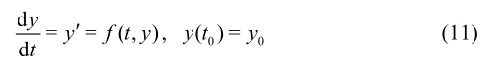
The solution can be advanced from tnto tn+1=tn+∆t by using the fifth-order Runge-Kutta formula derived:

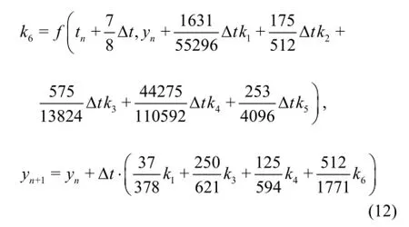
The fifth-order Runge-Kutta method evaluates the right-hand side derivatives five times per time step∆tand the final value yn+1is calculated based on these derivatives.

1.2.3 Dynamic mesh

The rotational velocity calculated by solving Eq.（10） are used to obtain the velocity of each moving boundary cell face

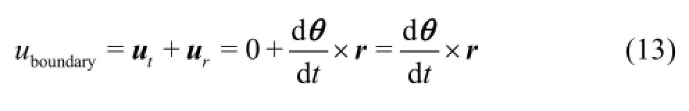
where utis the translational velocity which is zero in this study and uris the rotational velocity. Andr is the vector between the centre of the cell face and the COG. This velocity then is used to move the boundary， representing the surface of the rolling body.

The mesh motion of the computational domain is calculated by solving the cell-centre Laplace smoothing equation［20］

Here，γis the diffusion field anduis the point velocity used to modify the point positions of the mesh

where xoldand xneware the point positions before and after mesh motion and ∆tis the time step. The boundary motion obtained from Eq.（13） is used as boundary condition and then Eq.（14） is solved using the finite volume method （FVM） to diffuse the motion of the boundary to the whole computational domain.

Fig.1 Sketch of physical wave tank （m）

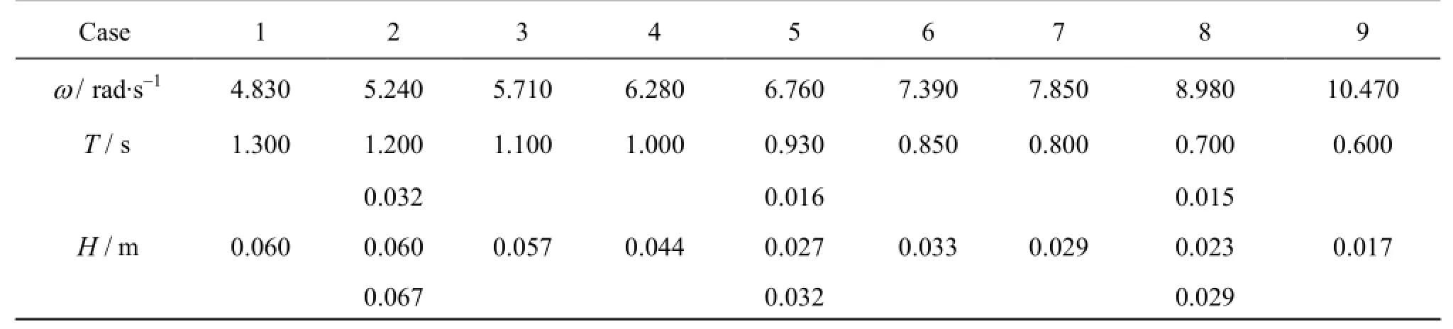
Table 1 Selected wave conditions

The variable diffusion fieldγis introduced to improve mesh quality［20］. There are two groups of diffusivity models supplied with OpenFOAM: the diffusion fieldγis a function of a cell quality measure and it is a function of cell centre distancel to the nearest selected boundary. The distance-based method is used together with the quality-based method. There are several sub-choices for each group of diffusivity models， details can be found in User's Guide of OpenFOAM［21］. In this study， the quality-based method inverseDistance and the distance-based method quadratic are selected. This means the diffusivity of the field is based on the inverse of the distance from the specified boundary， and the variable diffusion field γequals 1/l2.

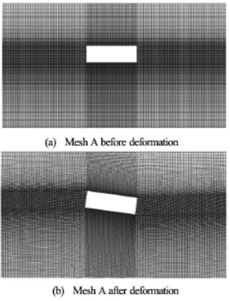
Fig.2 Multi-block grid system A around rectangular structure

1.3 Algorithm

Firstly， the computational domain is discretized into a number of arbitrary convex polyhedral cells. The valid mesh should be continuous， which means that the cells do not overlap with each other and fill the whole computational domain. The initial time step is specified as well. The Navier-Stokes Eq.（1） and （2） are then discretized into a set of algebraic equations based on the mesh. Then the following steps are carried out in each time step:

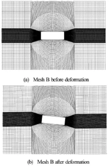
Fig.3 Multi-block grid system B around rectangular structure

Table 2 Mesh parameters and corresponding results

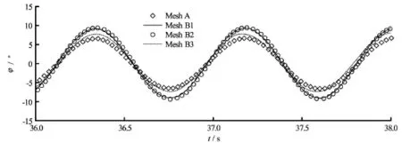
Fig.4 Mesh convergent test

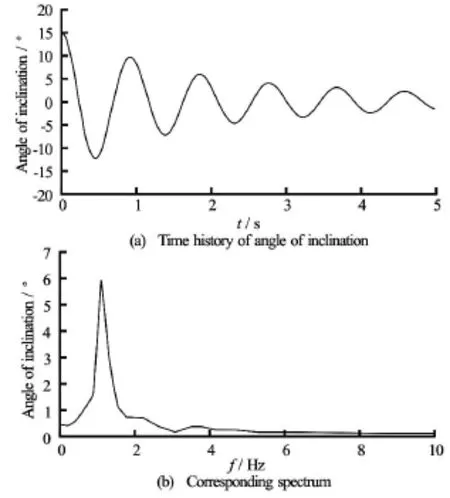
Fig.5 Test of roll free decay

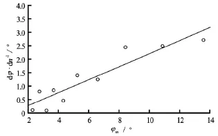
Fig.6 Curve of extinction of rolling

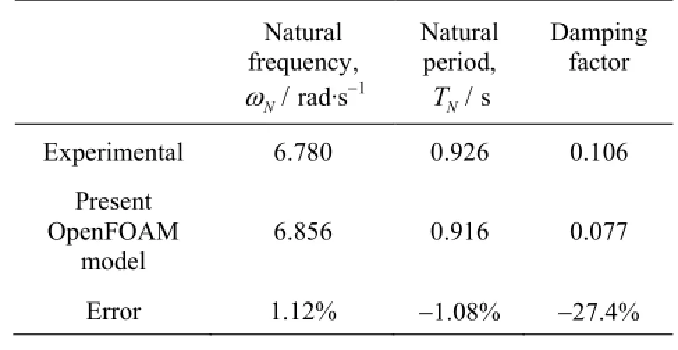
Table 3 Dynamic characteristics of roll motion

（2） The mesh motion equation Eq.（14） is solved to diffuse the motion of the boundary to the whole mesh.

（3） The volume fraction function is calculated by solving Eq.（3）.

Fig.7 RAO for roll motion

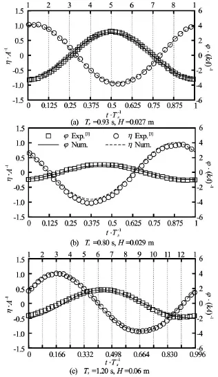
Fig.8 Time histories of wave elevation（η）of incoming waves and rotating angle of the rectangular structure（ϕ）at different wave periods and wave heights. Rotating angle and surface elevations are normalized by kA and A，respectively

（4） Navier-Stokes equations are solved based on the merged PISO-SIMPLE （PIMPLE） algorithm. The Semi-Implicit Method for Pressure-Linked equations（SIMPLE） algorithm allows the calculation of pressure on a mesh from velocity components by coupling the Navier-Stokes equations with an iterative procedure. The pressure implicit splitting operator （PISO） algorithm has been applied in the PIMPLE algorithm to rectify the pressure-velocity correction.

（5） The external moments are calculated by summing the moments about the COG over the body due to the pressure forces obtained by solving Eq.（1）and Eq.（8）.

（6） The equations of rigid body motions Eq.（10）are solved by applying the built-in ODE solver supplied with OpenFOAM. Then the new position of the moving boundary is determined.

2. Numerical results and discussions

The accuracy of the model in predicting the wave-induced roll motion is verified by comparing with the published experimental results collected by Jung et al.［3］. The effects of incident wave period， wave height and fluid viscosity on roll motions have been investigated as well as the influence of the size and draft of the floating structure on the natural frequency and the roll motion. The laminar flow model of OpenFOAM-2.1.0 is used in all computations in this paper. The cases presented in this paper were all run in parallel with 8 cores using the Aquila HPC system of the University of Bath. Generally， it would take about 49 h to simulate the roll motion for 40 s for cases with 2.14×106cells.

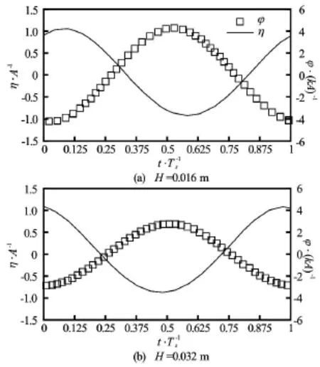
Fig.9 Time histories of wave elevation（η）of incoming waves and rotating angle of the rectangular structure（ϕ）at Ts=0.93swith different wave heights. Rotating angle and surface elevations are normalized bykAandA，respectively

2.1 Numerical wave tank

Experimental study on the roll motion of a 2-D rectangular barge in beam sea conditions presented by Jung et al.［3］has been selected in this study to validate and calibrate the extended OpenFOAM model. Once properly validated and calibrated， the code can be used to study the dependence of the roll motion on the surrounding sea states and the geometry of the floating structures.

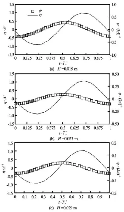
Fig.10 Time histories of wave elevation（η）of incoming waves and rotating angle of the rectangular structure（ϕ）at Ts=0.70swith different wave heights. Rotating angle and surface elevations are normalized bykA and A， respectively

In the experiments presented by Jung et al.［3］， a glass-walled wave tank （35 m×0.9 m×1.2 m） was used for the tests with a constant water depth of 0.9 m. A rectangular structure （0.3 m×0.9 m×0.1 m） with a draft that equals one half of its height was hinged at the center of gravity of the structure and it was allowed to roll but restrained from heave and sway motion （1 DoF）. A back-flap type wave maker was used to generate regular waves with wave periods ranging from T =0.5 s to 2.0 s， including the roll natural period（TN=0.93s）. Figure 1 shows the sketch of the tank. The wave parameters of selected cases in current analyses can be found in Table 1. Hereωis wave frequency andH is wave height. For the wave periods: T =0.70 s， 0.93 s and 1.2 s， i.e.，ω=8.98 rad/s，6.76 rad/s and 5.24 rad/s， the experiments were carried out with several different wave heights to study the effect of wave height on the roll motion.

In order to reproduce the experiments， a 2-D numerical wave tank is set-up. 2nd order Stokes' waves are generated at inlet boundary to hit the structure by applying Eqs.（5）-（7） for the water fraction at the inlet boundary. The velocities for the air fraction are set to zero. Noting that for the free-roll test described in the forthcoming section， the velocities of the water and air fraction of the inlet boundary are both set to zero. The top boundary is a pressure inlet/outlet，which allows air to leave or enter the computational domain. The empty condition is set to the sides of the model for which solutions are not needed， which is a built-in condition of OpenFOAM for front and back planes in 2-D simulations. The bottom is defined as a wall， which means the velocities of bottom are constrained to a value of zero. The far field boundary condition mentioned in Section 1 is applied at the downstream end of the tank to minimize reflections. The movingWallVelocity condition is applied to the moving rectangular barge to ensure that the flux across the structure is zero.

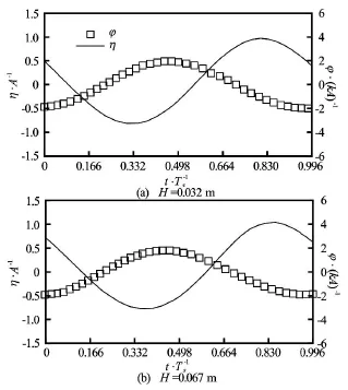
Fig.11 Time histories of wave elevation（η）of incoming waves and rotating angle of the rectangular structure（ϕ）at Ts=1.20swith different wave heights. Rotating angle and surface elevations are normalized bykA and A ， respectively

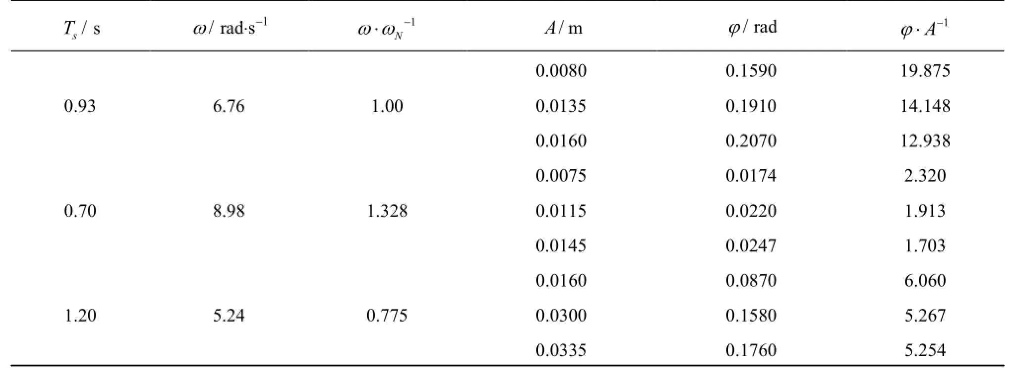
Table 4 Free surface elevation of incoming waves and rotating angle of the rectangular structure at three different periods with three different wave heights

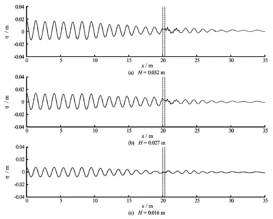
Fig.12 Wave profiles at the moment of t=40Tsfor Ts=0.93swith different wave heights and the dash ines represents the location of the floating object

Two different grid systems， referred to as Mesh A and Mesh B， were created by using BlockMesh， a built-in mesh generation utility supplied with OpenFOAM， as shown in Figs.2 and 3， respectively. In order to get better resolution of the flow field， the grid was refined in areas around the rectangular barge and the free surface. The refined area near the structure is different for Mesh A and Mesh B. The rectangular areas above and underneath the barge are refined in Mesh A while the circular area where the center sits on the COG of the barge with diameter of 0.6 m in Mesh B is refined. Three different meshes were generated based on the structured grid system Mesh B， shown in Fig.3， to assess the sensitivity of the model to the density of the mesh. These meshes were labelled as Mesh B1， Mesh B2 and Mesh B3. The mesh and wave parameters used for the convergence tests are summarized in Table 2 in which ∆x and ∆zrepresent the resolution in the horizontal and vertical direction， respectively. The time histories ofroll motion of the floating barge using four different meshes are shown in Fig.4 and their response amplitude operators （RAOs） are summarized and compared with the experimental result in Table 2 as well. It can be seen that the quality of the structured grid system Mesh B is higher than that of Mesh A by providing more accurate results even with coarser mesh. The grid dependence of the solutions in this study was not strong and thus， the medium grid system， Mesh B1，was selected for all cases shown in this paper.

Fig.13 Wave profiles at the moment of t=60Tsfor Ts=0.70swith different wave heights and the dash lines represents the location of the floating object

2.2 Dynamic characteristics of roll motion

A free-roll test was carried out to obtain the damping coefficient b and the natural angular frequency ωN， and the results are compared with the experiment［3］. The right-hand side in Eq.（10） vanishes because the test was performed in the calm water condition， and the equation of motion becomes［3］

whereξis the damping factor. The structure was initially inclined and released with an angle of 15o. There is no incoming wave and then the barge can roll freely with decaying roll amplitude.

The time history of the successively decaying roll amplitude was recorded and shown in Fig.5（a）. Then the natural frequency can be computed through the spectrum， shown in Fig.5（b）， obtained by applying the fast Fourier transform （FFT） analysis to the time history shown in Fig.5（a）. It can be seen from the graph that the natural frequency fN=1.092 Hzand then the natural angular frequencyωN=6.856 rad/s.

The formula of the damping coefficientbis given by［3］

where Tφis the natural rolling period and K1is the slope of the curve of extinction of rolling. The decrease in inclination for a single roll，dϕ/dn， and the total inclination，ϕm， are presented as an ordinate and an abscissa， respectively.dϕ/dnis the difference between two successive amplitude of the structure with the direction of inclination ignored andϕmis the mean angle of roll for a single roll. The curve of extinction of rolling is shown in Fig.6. From the graph we know thatK1=0.243and from the experiment， the mass of the structure is 13.5 kg andand we obtained from Eq.（18） thatb=0.377. Accordingly，the damping ratioζ=0.077.

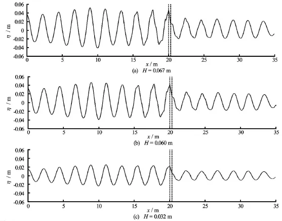
Fig.14 Wave profiles at the moment of t=30Tsfor Ts=1.20swith different wave heights and the dash lines represents the location of the floating object

The natural frequency， natural period and the damping ratio are summarized and compared with experimental results in Table 3. The natural frequency matches well with experiments while there is a relative large discrepancy for damping ratio which is likely due to 2-D flow assumption and frictional damping of hinges introduced in experiments. In addition， the turbulence model is not used in order to reduce computation time.

2.3 Roll motion of a 2-D rectangular barge in presence of waves

2.3.1 Roll motion and wave profiles

Variations of the magnification factors （ϕ/kA，also called the RAOs， in whichϕis the angle of roll，k is wave number and Ais wave amplitude） of the barge with the dimensionless wave frequencies（ω/ ωN）were first examined. The numerical results have been compared with the experimental data and the available theoretical solutions based on linear potential flow theory［3］， shown in Fig.7. It can be seen that the numerical results from the extended OpenFOAM model agree well with experiments in general. However， the roll motion calculated using linear potential flow theory given in the paper［3］is significantly overpredicted at the natural frequency due to the assumption that the fluid is inviscid and irrotational， i.e.， the potential flow theory only considers wave making damping but not viscous damping. Additionally， at lower frequencies （ω/ ωN＜0.8）， the potential flow theory underestimates the magnification factors compared to the experimental and numerical results. The possible reason is that the viscous effect neglected in potential flow theory helps to increase the roll at lower frequencies.

The time histories of roll angle of the rectangular structure（ϕ）and free surface elevation of incoming waves（η）for different wave periods of Ts=0.93 s， 0.8 s and 1.2 s in one periods of the wave， in which the wave has been fully developed and reaches its stable state， have been plotted in Fig.8 together with those from the experiments conducted by Jung et al.［3］. It can be seen that the present numerical model can predict the flow fields and wave-induced roll motion accurately regardless of the wave periods， with close matching of both the shape and crest values of free surface elevation and roll motion of the rectangular barge. As expected， due to the resonance effect， the amplitude ofϕis largest for the case with Ts=0.93s，which is very close to the natural period of the rectangular barge， 0.926/0.916 s， shown in Table 2， even with smallest wave height of the incoming wave.

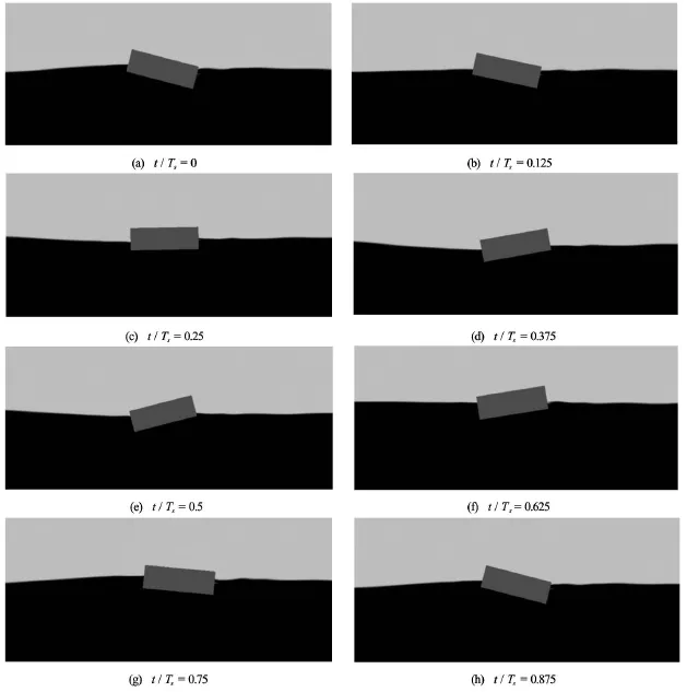
Fig.15 2-D views of Ts=0.93s，H=0.032 mwave hitting on the structure: phase number of each subtitle matches to the phase in Fig.9（a）

In order to further investigate the effect of wave height on the roll motion， the time histories of φ and η with different wave heights at Ts=0.93 s， 0.7 s and 1.2 s， corresponding toω/ ωN=1， 1.328 and 0.775，are shown in Figs.9-11， respectively. Comparisons show that the roll motion increases with the increase of wave height regardless of the wave period. While the trend of RAO values for different wave periods is different. It decreases with the increase of wave height at the natural frequency （Ts=0.93sor ω/ ωN=1），while has the similar values at different wave heights for wave frequencies away from the natural frequency（Ts=0.7 s and 1.2 s or ω/ ωN=1.328 and 0.775），shown in Fig.7 as well. The crest values of free surface elevation and rotating angle are highlighted in Table 4. It confirms that the increment in free surface elevation and roll motion is similar except for cases with the natural wave period， which means that the nonlinear effect on the roll damping is significant only for the natural frequency. Additionally， phase difference is observed for cases at the same wave frequency but with different wave heights.

Figures 12-14 show wave profiles along the central line of the tank for different wave periods of Ts= 0.93 s， 0.7 s and 1.2 s， respectively and each with three different wave heights. For all three periods，phase difference can be observed， especially at Ts= 0.7 s， consistent with what is observed from Figs.9-11. There is significant difference between the wave on the seaward and leeward sides of the structure which would determine the behaviour of the forces impacting on the structure. This will be discussed in more details in the following section. In addition， it can beseen that the nonlinearity of the wave behind the structure is stronger for the cases with natural wave period than that at wave periods away from the natural wave period. In order to give more vivid impressions， Fig.15 shows several snapshots of the 2-D wave field around the structure for the case with Ts=0.93s，H= 0.032 m according to phases， as shown in Fig.8（a）.

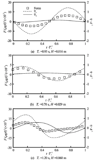
Fig.16 Time history of horizontal forces and forces and surface elevations are normalized by ρgAandA， respectively. （solid line: wave behind structure， dash line: wave at the front of structure， rectangular symbol: horizontal force）

2.3.2 Forces impacting on the structure

The horizontal （Fx）and vertical forces （Fz）impacting on the rectangular structure are shown in Fig.16 and Fig.17， respectively， together with the wave elevations of ηsand ηLon the seaward and leeward sides at different wave periods in one periods. It can be seen that regardless of the wave periods， the positive values of∆η=ηs-ηLlead to positive forces and vice versa， which means that the sign and magnitude of forces are determined by the difference in wave elevations at the left and right hand side of the structure. Especially， in the cases of Ts=0.93sand Ts=0.70s，the time behaviour of forces are mainly determined by the change ofηson the seaward side due to the little variation inηLas shown in Figs.16（a）-16（b） and Figs.17（a）-17（b） for Ts=0.93sand Ts=0.7 s， respectively.

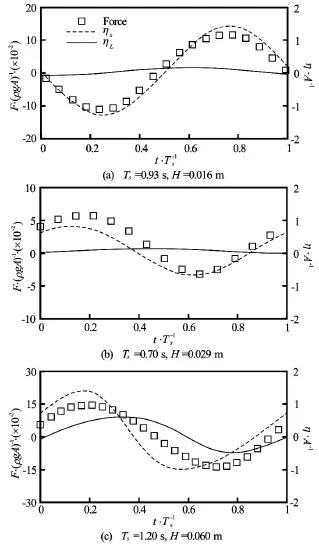
Fig.17 Time history of vertical forces and forces and surface elevations are normalized by ρgAandA， respectively. （solid line: wave behind structure， dash line: wave at the front of structure， rectangular symbol: vertical force）

The relation between forces and the difference in wave elevations on the seaward and leeward sides with respect to the wave height has been studied and shown in Figs.18， 19， Figs.21， 22 and Figs.24， 25 for Ts= 0.93 s，Ts=0.70sand Ts=1.20s， respectively. Not surprisingly， the time behaviour of forces impacting on the structure is independent of the wave heights of the incoming waves for all three wave periods while is determined by the difference in wave heights of the wave on the seaward and leeward sides of the structure. It is interesting to find that the normalized forces in both horizontal and vertical direction have similarvalues at different wave heights even for cases with Ts=0.93s， which is very close to the roll natural period of the rectangular structure， as shown in Fig.20， Fig.23 and Fig.26 for Ts=0.93s，Ts=0.70sand Ts=1.2s， respectively. This means that the nonlinear effect for wave loading is less significant when compared with wave-induced roll motion. Additionally， as with wave elevation and roll motion， phase difference in wave loading at different wave heights is observedand for all three wave periods， the phase difference in the case of Ts=1.20sis the smallest， consistent with what has been observed in Figs.12-14.

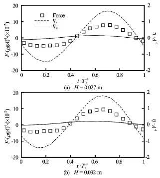
Fig.18 Time history of horizontal forces for Ts=0.93sand forces and surface elevations are normalized byρgA and A， respectively. （solid line: wave behind structure，dash line: wave at the front of structure， rectangular symbol: horizontal force）

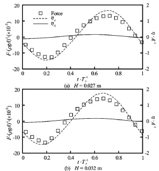
Fig.19 Time history of vertical forces for Ts=0.93sand forces and surface elevations are normalized byρgA andA ， respectively. （solid line: wave behind structure，dash line: wave at the front of structure， rectangular symbol: horizontal force）

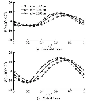
Fig.20 Time history for Ts=0.93swith various wave heights and forces are normalized byρgA

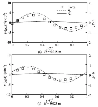
Fig.21 Time history of horizontal forces for Ts=0.70sand forces and surface elevations are normalized byρgA andA， respectively. （solid line: wave behind structure，dash line: wave at the front of structure， rectangular symbol: horizontal force）

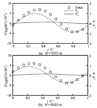
Fig.22 Time history of vertical forces for Ts=0.70sand forces and surface elevations are normalized byρgAand A， respectively. （solid line: wave behind structure， dash line: wave at the front of structure， rectangular symbol: horizontal force）

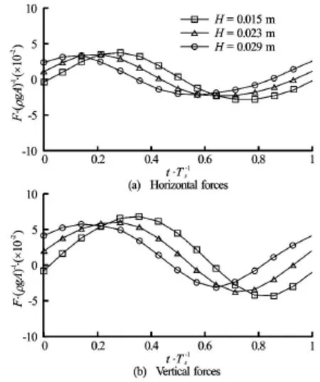
Fig.23 Time history for Ts=0.70swith various wave heights and forces are normalized byρgA

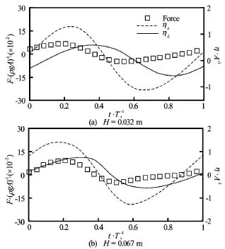
Fig.24 Time history of horizontal forces for Ts=1.20sand forces and surface elevations are normalized byρgA and A， respectively. （solid line: wave behind structure，dash line: wave at the front of structure， rectangular symbol: horizontal force）

Fig.25 Time history of vertical forces and forces and surface elevations are normalized by ρgAandA， respectively. （solid line: wave behind structure， dash line: wave at the front of structure， rectangular symbol: horizontal force）

The maximum and minimum values of both horizontal and vertical forces for all three wave periods，Ts=0.93s，H =0.027 m，Ts=0.70s，H=0.029 m and Ts=1.20s，H=0.06 m， are summarized in Table 5. The forces are normalized byρgA，Ais the wave amplitude. Generally， the magnitude of forcesincreases with the increase of wave periods， while the variations between the cases with the natural period of Ts=0.93sand the longer wave period of Ts=1.20s is not significant.

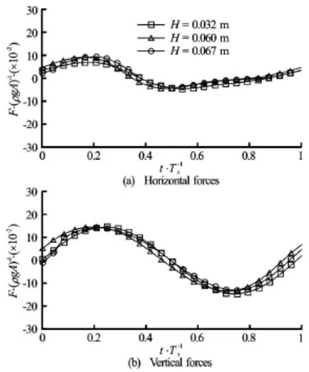
Fig.26 Time history for Ts=1.20swith various wave heights and forces are normalized byρgA

A study has been conducted in order to determine the relation of wave loading hitting fixed and floating structures with the same cross section in the same sea conditions， as shown in Fig.27. This suggests that for all the cases considered the wave loading on fixed structures has close matching in both crest values and the shapes with those of floating structures.

2.3.3 Velocity and vorticity fields

An interesting finding in Fig.7 is that the RAOs obtained from the linear potential-flow theory agree well with those obtained from the experiments and viscous-flow solver for shorter waves （ω＞ωN）， but the linear potential theory clearly underestimates the RAOs for longer waves（ω＜ωN）. Further investigations have been carried out for long wave with period ofTs=1.20sto explain this phenomena. The velocity and vorticity fields ofTs=1.20s（ω/ ωN=0.775），H=0.032 mwave close to both sides of the 2-D barge are shown in Fig.28. Subplots in Fig.28 are named from （a） to （l）， which matches the phases of the roll motion shown in Fig.8（c）. The barge reaches its maximum clockwise motion at Fig.28（a） and experienced counter-clockwise motion from Figs.28（b）-28（g）. It can be seen from Fig.28（a） that the negative vortex（black） exists at the seaward side of the structure and after a short period of time， the negative vortex （black） diffuses and a positive vortex （white） appears and is staying during the rollaway motion from Figs.28（b）-28（g）. At the right hand side of the structure， the positive vortex （white） decays and the negative vortex（black） increases during the rollaway cycle. The barge reaches its maximum counter-clockwise position at Fig.28（h） and experiences clockwise motion from Figs.28（i）-28（l）. Similar to the counter-clockwise motion， the positive vortex diffuses quickly and a negative vortex develops at the left hand side of the structure. In contrast to the seaward side， the negative vortex decays while the positive vortex appears and is remaining during the roll-in cycle near the left bottom corner on the leeward side. A similar mechanism was observed by Jung et al.［3］and they explained that since the position of the positive vortex is “ahead” of the rolling direction of the structure during most of the cycle， the structure experiences “negative” damping，i.e.， the viscous effect increases the roll motion at lower frequencies rather than damping it out which is observed in Fig.7.

2.3.4 Parametric studies

Numerical studies have been carried out to investigate the dependence of roll motion on body draft，height and breadth. The cross section used in previous section or experiments described by Jung et al.［3］is chosen as standard case， and the depth and breadth of the object are labelled asD andB， respectively. A new parameterε， the ratio in characteristic length of new cross sections and the standard case， is introduced to describe the change in cross section and draft. That is，ε=d/ D，a/ Dand b/ Bfor cases with various drafts， body heights and body widths， respectively. Here，d，aandbrepresent the depth of the body under the water surface， one half of depth and width of new cross sections， respectively.

2.3.5 Influence of body draft

In order to investigate the influence of body draft on the roll motion， three different drafts ε=d/ D= 0.375， 0.500 and 0.625 are considered with the same body breadth B =0.3mand body height D =0.1m. ε=0.500means that the structure is half submerged. Variations of the magnification factors of the rectangular barge with the incident wave frequenciesωfor all three drafts are shown in Fig.29. It can be seen that the roll motions for a 2-D rectangular barge increase gradually withωat lower frequencies and reach its maximum between ω=6.4 rad/sand ω=7.4 rad/s for differentε. The roll motions then decrease with the increase of theωafterwards. Additionally， the natural frequency ωN， corresponding response frequency of the maximal roll motion， tends to decrease with the increase of body draft and the peak value of the roll motion for the casesε=0.500is the largestamong three drafts and the smallest roll motion occurs when ε=0.375. Generally， the roll motions at lower frequencies are larger than those at higher frequencies. For waves with lower frequencies， the roll motions for ε=0.625are larger than those of ε=0.375cases and cases withε=0.500sit in between. However，for waves with higher frequencies， the trend is opposite， i.e.， the roll motions forε=0.625are smaller than those ofε=0.375cases. It means that for longer wave conditions， the deep-draft barge is less stablethan the shallow-draft barge， and vise versa for shorter wave， which is consistent with the conclusions presented by Chen et al.［22］. They argued that in order to minimize the wave-induced roll motion， engineers from oil and gas industry or ship companies need to adjust the deck loading so that the natural frequency can be moved away from the dominant frequency of the ambient sea conditions.

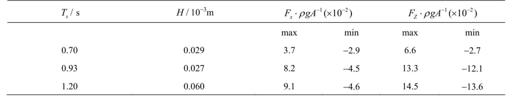
Table 5 The maximum and minimum of the horizontal and vertical forces

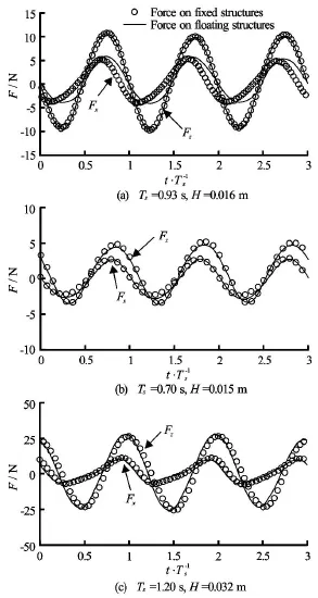
Fig.27 Time history of forces on fixed rectangular （solid line）and rotating rectangular （○）

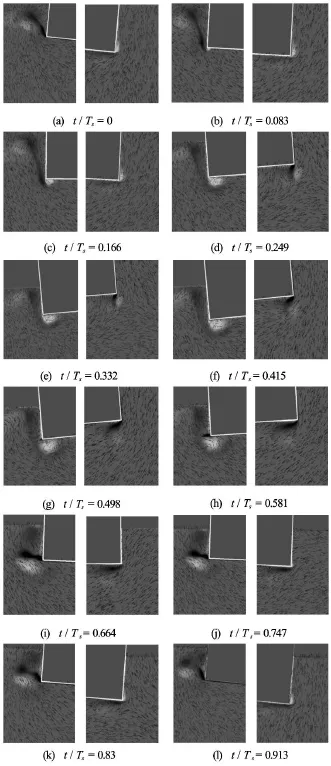
Fig.28 Vorticity and velocity field of Ts=1.20s，H= 0.032 m wave: phase number of each subtitle matches to the phase in Fig.9（c）

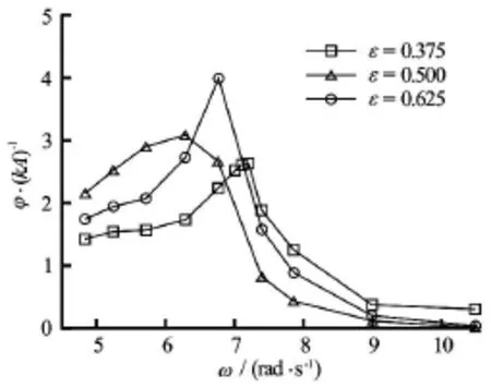
Fig.29 Magnification factors for roll motion for cases with all three drafts （ε=　d/ D，d is draft andDis depth of the object）

Fig.30 Magnification factors for roll motion for cases with all three body heights （ε=　a/ D，ais half of depth of the object）

2.3.6 Influence of body height

The variation of roll motion with the incident wave frequenciesω， concerning the influence of body height is investigated in this section. Three body heights are considered， i.e.，ε=a/ D=0.375， 0.500 and 0.625 with the same draftd=0.05 mand body breadthB=0.3m. Variations of the magnification factors of the rectangular barge with the incident wave frequenciesωfor all three body heights are shown in Fig.30. Similar trends to cases concerning the influence of body draft are observed. It can be seen from Fig.30 that the motions increase gradually with the increase ofωand reach their maximum at the natural frequencies， which decrease with the increase of body height. Again， the maximum and minimum peak values of the roll motion are observed when ε=0.500 and ε=0.375among cases with all three body heights， respectively. The roll motions at lower frequencies are generally larger than those at higher frequencies. And at lower frequencies， the larger the body height is the larger the roll motion， and vise versa for waves with higher frequencies.

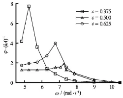
Fig.31 Magnification factors for roll motion for cases with all body width （ε=　b/ B，b is half of width of the object，Bis the width of the object）

2.3.7 Influence of body breadth

The influence of body breadth on the natural frequency and the roll motion of a 2-D barge is studied here with three different body breadths， i.e.，ε=0.375，0.500 and 0.625 with the same draftd=0.05 mand body heightD=0.1m. Variations of the RAOs of the rectangular barge with the incident wave frequenciesωfor all three body breadth are shown in Fig.31. It can be seen from the graph that the roll motions increase gradually with the increase of ω until reach the maximum values at the natural frequencies and the roll motions at lower frequencies are larger than those at higher frequencies， which are also observed in Figs.29 and 30. The natural frequency for cases with smaller breadth is lower than those with larger breadth while the trend for the corresponding roll motion is opposite， i.e.， the peak value of the roll motion for ε=0.375is the largest. Additionally， the roll motions for the cases with smaller body breadth is larger than those with larger body breadth for longer wave conditions， and vise versa for shorter waves.

3. Conclusions

OpenFOAM has been further extended and used in the present study to model the roll motion of a 2-D rectangular barge under wave actions. The modules developed in Ref.［14］ have been selected here for wave generation and absorbing. The wave generation is via the flux into the computational domain through a vertical wall. The velocities from the 2nd order Stokes' wave theory are used for generating regular waves and the numerical beach is applied to minimizewave reflection at the end of the wave tank. The viscous-flow solver for multiphase problems with moving mesh， interDyMFoam， supplied with OpenFOAM， has been extended for predicting roll motions of floating structures. The new locations of the floating structures are determined by solving the equations of motion using the ODE solver supplied with OpenFOAM based on fifth-order Cash-Karp Runge-Kutta method.

Comparisons among the present numerical results，potential-flow results given in the paper［3］and the measured data collected by Jung et al.［3］have indicated that the extended OpenFOAM used in the present study is very capable of accurate modelling of wave interaction with freely rolling structures， with the natural frequency and roll motion correctly captured. However， the potential flow theory over-predicts the roll motion significantly at the natural frequency and underestimates the roll motion at lower frequencies due to the fact that the viscous damping is not taken into account in the potential flow theory.

The roll motion increases gradually with the increase of the incident wave frequency until reach its maximum values at the natural frequency. It is also found that at the natural frequency， the magnification factors for roll motion decrease with the increase of the incident wave height while for wave frequencies away from the natural frequency， the magnification factors have the similar values， i.e.， the nonlinear effect on the roll damping is significant only for the natural frequency. With respect to the wave loading on the structures， the time behavior of normalized forces are determined by the difference in wave free surface elevations on the seaward and leeward sides of the structure regardless of wave periods and wave heights of incoming waves. Additionally， the investigation on the velocity and vorticity fields reveals that the viscous effect not only can damp out the roll motion but also can help the structure to roll.

The parametric study has been carried out to shed some insight on the influence of body draft， height and breadth on the roll motion of a 2-D rectangular barge. These new results have revealed that the natural frequency increases with the increase of body breadth while decreases with the increase of body draft and height. The largest peak values of the roll motion at the natural frequency are observed for the cases with the smallest body breadth or for the cases with medium body draft and height. Moreover， at lower frequencies，the roll motion is generally larger than that at higher frequencies.

Acknowledgments

Authors are very grateful for the reviewers' constructive comments and suggestions， which have helped to improve the quality of this paper. The first author acknowledges the financial support of the University of Bath and China Scholarship Council （CSC）for her Ph. D. study. Authors are also grateful for the use of the HPC facility at University of Bath for some of the numerical analysis.

References

［1］ SURENDRAN S.， VENKATA RAMANA REDDY J. Numerical simulation of ship stability for dynamic environment［J］. Ocean Engineering， 2003， 30（10）: 1305-1317.

［2］ TAYLAN M. The effect of nonlinear damping and restoring in ship rolling［J］. Ocean Engineering， 2000， 27（9）: 921-932.

［3］ JUNG K. H.， CHANG K. A. and JO H. J. Viscous effect on the roll motion of a rectangular structure［J］. Journal of Engineering Mechanics， 2006， 132（2）: 190-200.

［4］ WU X.， TAO L. and LI Y. Nonlinear roll damping of ship motions in waves［J］. Journal of Offshore Mechanics and Arctic Engineering， 2005， 127（3）: 205-211.

［5］ LEE J. H.， INCECIK A. The simplified method for the prediction of radiation damping coefficients［C］. Proceedings of the 16th International Offshore and Polar Engineering Conference. Lisbon， Portugal， 2007， 2178-2183.

［6］ CHAKRABARTI S. Empirical calculation of roll damping for ships and barges［J］. Ocean Engineering， 2001， 28（7）: 915-932.

［7］ KAWAHARA Y.， MAEKAWA K. and IKEDA Y. A simple prediction formula of roll damping of conventional cargo ships on the basis of Ikeda's method and its limitation［J］. Fluid Mechanics and its Applications， 2011， 97: 465-486.

［8］ ZHAO X.， HU C. Numerical and experimental study on a 2-D floating body under extreme wave conditions［J］. Applied Ocean Research， 2012， 35（1）: 1-13.

［9］ BANGUN E. P.， WANG C. M. and UTSUNOMIYA T. Hydrodynamic forces on a rolling barge with bilge keels［J］. Applied Ocean Research， 2010， 32（2）: 219-232.

［10］ WILSON R. V.， CARRICA P. M. and STERN F. Unsteady RANS method for ship motions with application to roll for a surface combatant［J］. Computers and Fluids， 2006，35（5）: 501-524.

［11］ CHEN H. C.， LIU T. and CHANG K. A. Time-domain simulation of barge capsizing by chimera domain decomposition approach［C］. Proceedings of the 12th International Offshore and Polar Engineering Conference. Kitakyushu， Japan， 2002.

［12］ MORGAN G.， ZANG J. and GREAVES D. et al. Using the rasInterFoam CFD model for wave transformation and coastal modeling［C］. Proceedings of 32nd Conference on Coastal Engineering. Shanghai， China， 2010.

［13］ MORGAN G.， ZANG J. Application of OpenFOAM to coastal and offshore modelling［C］. The 26th IWWWFB. Athens， Greece， 2011.

［14］ CHEN L. F.， ZANG J. and HILLIS A. J. et al. Numerical investigation of wave-structure interaction using OpenFOAM［J］. Ocean Engineering， 2014， 88: 91-109.

［15］SUN L.，CHEN L. F. and ZANG J.et al.Nonlinear interactions of regular waves with a truncated circular column［C］. ITTC Workshop on Wave Run-up and Vortex Shedding. Nantes， France， 2013.

［16］ EKEDAHL E. 6-DOF VOF-solver without damping in OpenFOAM［R］. Project work for the Ph. D. course “CFDwith Open Source Software”， Gothenburg， Sweden: Chalmers University of Technology， 2008.

［17］ YOUSEFI R.， SHAFAGHAT R. and SHAKERI M. Hydrodynamic analysis techniques for high-speed planning hulls［J］. Applied Ocean Research， 2013， 42: 105-113.

［18］ RUSCHE H. Computational fluid dynamics of dispersed two-phase flows at high phase fractions［D］. Doctoral Thesis， London， UK: Imperial College London， 2003.

［19］ De BRUIJUN R.， HUIJS F. and HUIJSMANS R. et al. Calculation of wave forces and internal loads on a semisubmersible at shallow draft using an IVOF method［C］. Proceedings of the ASME 2011 30th International Conference on Ocean， Offshore and Arctic Engineering. Rotterdam， The Netherlands， 2011.

［20］ JASAK H.， TUKOVIC Z. Automatic mesh motion for the unstructured finite volume method［J］. Transactions of Famena， 2006， 30（2）: 1-20.

［21］ The OpenFOAM® Foundation. The open source CFD toolbox of OpenFOAM: User Guide［M］. OpenCFD Ltd，2011.

［22］ CHEN H. C.， LIU T. and HUANG E. T. Time-domain simulation of large amplitude ship roll motions by a chimera RANS method［C］. Proceedings of the 11th International Offshore and Polar Engineering Conference. Stavanger， Norway， 2001.

10.1016/S1001-6058（16）60659-5

January 27， 2015， Revised July 1， 2015）

* Biography: Lifen CHEN （1987-）， Female， Ph. D.，Research Fellow

2016，28（4）:544-563