New prospects for computational hydraulics by leveraging high-performance heterogeneous computing techniques*

Qiuhua LIANG, Luke SMITH, Xilin XIA

1. Hebei University of Engineering, Handan 056038, China

2. School of Civil Engineering and Geosciences, Newcastle University, Newcastle upon Tyne, UK,

E-mail: Qiuhua.Liang@ncl.ac.uk

New prospects for computational hydraulics by leveraging high-performance heterogeneous computing techniques*

Qiuhua LIANG1,2, Luke SMITH2, Xilin XIA2

1. Hebei University of Engineering, Handan 056038, China

2. School of Civil Engineering and Geosciences, Newcastle University, Newcastle upon Tyne, UK,

E-mail: Qiuhua.Liang@ncl.ac.uk

In the last two decades, computational hydraulics has undergone a rapid development following the advancement of data acquisition and computing technologies. Using a finite-volume Godunov-type hydrodynamic model, this work demonstrates the promise of modern high-performance computing technology to achieve real-time flood modeling at a regional scale. The software is implemented for high-performance heterogeneous computing using the OpenCL programming framework, and developed to support simulations across multiple GPUs using a domain decomposition technique and across multiple systems through an efficient implementation of the Message Passing Interface (MPI) standard. The software is applied for a convective storm induced flood event in Newcastle upon Tyne, demonstrating high computational performance across a GPU cluster, and good agreement against crowdsourced observations. Issues relating to data availability, complex urban topography and differences in drainage capacity affect results for a small number of areas.

computational hydraulics, high-performance computing, flood modeling, shallow water equations, shock-capturing hydrodynamic model

Introduction

Computational hydraulics is the field of developing and applying numerical models to solve hydraulic problems. It is a synthesis of multiple disciplines including but not restricted to applied mathematics, fluid mechanics, numerical analysis and computer science. The field has undergone rapid development in the last three decades, particularly following the advances in remote sensing technology, facilitating a rich source of topographic and hydrological data to support various modeling applications. Full 2-D and even 3-D numerical models have been developed to predict complex flow and transport processes and applied to simulate different aspects of hydrosystems, particularly flood inundation in extended floodplains. However, due to the restrictions in computational power, the app-lication of these sophisticated models has long been restricted to performing simulations in relatively localized domains of a limited size.

Taking 2-D flood modeling as an example, considerable research effort has been devoted to improving the computational efficiency of flood models, in order to allow simulations at higher spatial resolutions and over greater extents. The common approaches that have been attempted include simplifying the governing equations, improving the numerical methods and developing parallel computing algorithms. Simplified 2-D hydraulic models with kinematic- or diffusivewave approximations for flood inundation modeling had dominated the literature in the first decade of the 21st century[1-3]. These published works have shown that in certain cases these simplified models can reproduce reasonably well the flood extent and depth with high computational efficiency. However, accurate prediction of the evolution of flood waves involving complex processes is impossible without accurate representation of hydrodynamic effects, and is beyond the capabilities of these simplified models. Their reduced physical complexity may also cause increasedsensitivity to, and dependence on parameterization[4,5]. Furthermore, the reduction of computational time by these simplified approaches is not consistent across simulations, but highly dependent on the simulation resolution and flow hydrodynamics of the application[6,7].

Computationally more efficient numerical methods, including dynamically adaptive grids and subgrid parameterization techniques, have also been widely developed to improve computational efficiency. Adaptive grids can adapt to the moving wet-dry interface and other flow and topographic features, thus facilitate accurate prediction of the flood front and routing processes. By creating a refined mesh only in areas of interest, dynamic grid adaption provides an effective means to relax the computational burden inherent in full dynamic inundation models[8,9]. However, since the time step of a simulation is controlled by the cells with highest level of refinement, which is concentrated on the most complex flow dynamics and highest velocities or free-surface gradients, the speedup achieved through adaptive grid simulation is generally limited, typically up to ～3 times for practical applications.

Rather than creating high-resolution mesh to directly capture small-scale topographic or flow features, as used in the adaptive mesh methods, techniques known as sub-grid parameterization have also been developed to integrate small aspects of topographic features into flood models, to enable more accurate and efficient but still coarse-resolution simulations[10,11]. For example, Soares-Frazão et al.[10]introduced a new shallow flow model with porosity to account for the reduction in storage due to sub-grid topographic features. The performance of the porosity model was compared with that of a refined mesh model explicitly reflecting sub-grid scale urban structures, and a more classical approach of raising local bed roughness. While being able to reproduce the mean characteristics of urban flood waves with less computational burden than refined mesh simulations, the porosity model was unable to accurately predict the formulation and propagation of certain localized wave features, e.g. reflected bores.

Parallel programming approaches have also been adopted to facilitate more efficient hydraulic simulations, and shown to exhibit good weak and strong scaling when software is structured appropriately[12,13]. However, none of the above three approaches has proven to be truly successful until the advent of heterogeneous computing leveraging graphics processing units (GPUs). GPUs are designed to process large volumes of data by performing the same calculation numerous times, typically on vectors and matrices. Such hardware architectures are well-suited to the field of computational fluid dynamics. New programming languages including CUDA and OpenCL have exposed this hardware for use in general-purpose applications (GPGPU). A number of attempts have been made to explore the benefits of GPU computing for highly efficient large-scale flood simulations. Early pioneers of such methods include Lamb et al.[14]who harnessed graphics APIs directly to implement a diffusion wave model (JFlow) for GPUs, Kalyanapu et al.[15]with a finite-difference implementation of the full shallow water equations, and later Brodtkorb et al.[16]with a finite-volume scheme. Such software is becoming increasingly mainstream, Néelz and Pender[17]report results from several commercial GPU hydraulics implementations while Smith and Liang[18]demonstrate the potential for generalized approaches applicable to both CPU and GPU co-processors. The most recent research also explores how domain decomposition across multiple GPUs can provide further performance benefits[19].

This work presents a hydrodynamic model, known as the High-Performance Integrated Modelling System (HiPIMS), for simulating different types of natural hazards (results are presented for flood modelling herein). HiPIMS solves the 2-D shallow water equations (SWEs) using a first-order or second-order shock-capturing finite-volume Godunov-type numerical scheme although only the first-order scheme is used in this work. To substantially improve computational efficiency, the model is implemented for highperformance heterogeneous computing using the OpenCL programming framework, and therefore can take advantage of either CPUs or GPUs with a single codebase. The model has also been developed to support simulations across multiple GPUs using a domain decomposition technique and across multiple systems through an efficient implementation of the Message Passing Interface (MPI) standard. The unprecedented capability of HiPIMS to achieve high-resolution large-scale flood inundation modeling at an affordable computational cost is demonstrated through an application to reproduce the June 2012 Newcastle flood event. Two simulations have been carried out with a 2 m resolution, one covering 36 km2of Newcastle central area and another covering 400 km2of Tyne and Wear, which respectively involve 8×106and 108computational cells.

1. HiPIMS-a high-performance shallow flow model

HiPIMS solves the matrix form of the 2-D SWEs with source terms, given as follows

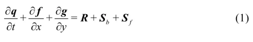
wheret is time,xandyare the Cartesian directions,qis the vector containing the conserved flowvariables,f and gare the flux vector terms in the two Cartesian directions,R,Sband Sfrepresent the source terms of rainfall, bed slope and friction. The vector terms are given by

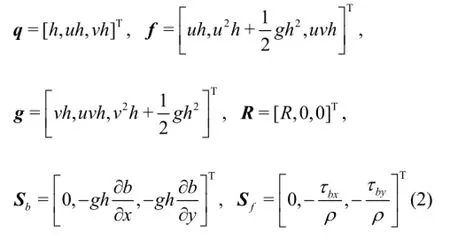
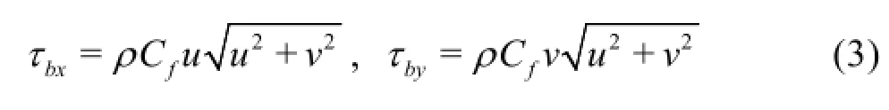
where uandvare the two Cartesian velocity components,h =η-b is the total water depth with η and brespectively denoting the water surface elevation and bed elevation above datum,gis the acceleration due to gravity,R is the rainfall rate,ρis the water density, and tbxand tbyare the friction stresses estimated using the Manning formula as follows

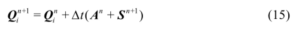
The above SWEs are numerically solved using a first-order finite volume Godunov-type scheme on Cartesian uniform grids. The corresponding time marching formula for updating the flow variables at an arbitrary celliis

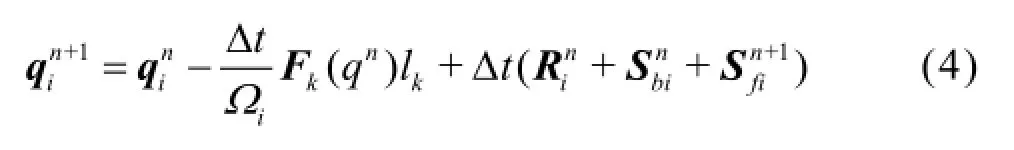
where n represents the time level,∆tis the time step,Ωiis the area occupied by celli,kis the index of the cell edges (N=4for the Cartesian uniform grids as adopted in this work),lkis the length of cell edge k,contains the fluxes normal to the cell edge andis the unit vector defining the outward normal direction. The currently adopted numerical scheme discretizes explicitly the flux term F and slope source term Sb. But the friction source term Sfis evaluated implicitly to achieve the so-called strongly AP scheme[20]to reproduce, to certain extent, the “asymptotic” behavior of the governing equations. This is an essential step to ensure the numerical scheme to correctly represent the physical processes of overland flows and guarantee numerical stability when water depth becomes small.

In Eq.(4), the interface fluxes Fk( q)are obtained by solving local Riemann problems in the context of a Godunov-type scheme. This requires the reconstruction of the Riemann states from the cell center values of the flow variables to define the local Riemann problems across the cell interfaces. HiPIMS adopts the surface reconstruction method (SRM) as proposed by Xia et al.[21], which firstly finds the water surface elevation at the cell interfaces to support the derivation of the final Riemann states. Considering two neighboring cells “i ” and “i+1”, SRM reconstructs the water surface elevation at left and right hand sides of the common cell interface through

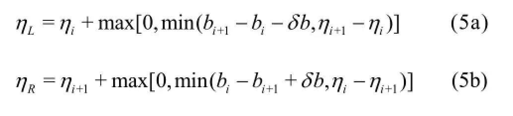
with

in which bi+1/2+and bi+1/2-are corresponding values of bed elevation at the right and left hand sides of the cell interface, which is obtained through a slope-limited linear reconstruction approach

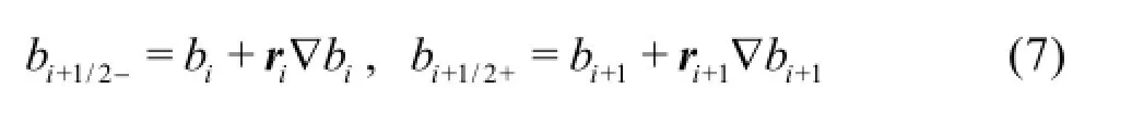
wherer is the distance vector defined as from the cell center to central point of the cell interface under consideration,∇brepresents the slope-limited bed gradient and a minmod slope limiter is used herein.

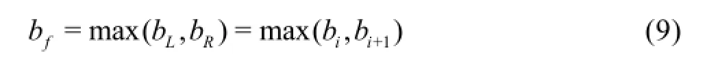
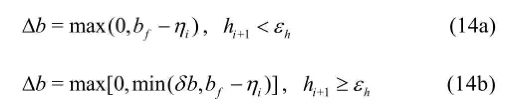
With the reconstructed water surface elevations provided by Eq.(5), the corresponding bed elevations at left and right hand sides of the cell interface can be obtained

from which a single face value of bed elevation is defined at the cell interface as a key step to derive the final Riemann states for implementation of the hydrostatic reconstruction method[22]

Subsequently, the Riemann states of water depth are defined as follows

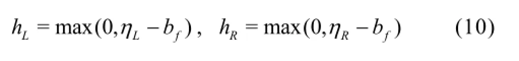
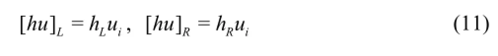
This ensures non-negative water depth and supports the derivation of the Riemann states of other flow variables, i.e. unit-width discharges

With the Riemann states provided by Eqs.(10)-(11), the interface fluxes across all four interface of the cell under consideration can now be evaluated using a Riemann solver and the HLLC approximate Riemann solver is employed in this work (see Ref.[23] for detailed implementation). The bed slope source terms can be simply discretized using a central difference scheme

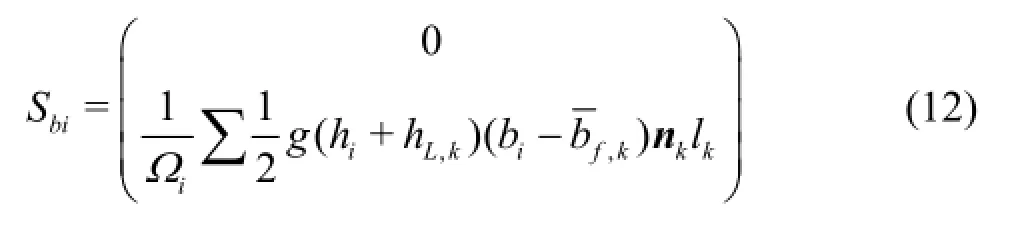
where hL,kis the left Riemann state of water depth at cell edgek, andis defined as

with

where εhis a infinitesimal value to define a dry cell, taken as 10-10in this work.

As mentioned previously, this work implements an implicit scheme to discretize the friction source terms in order to develop a “strongly AP scheme”. It is only necessary to consider the momentum equations here as the continuity equation does not involve a nonzero friction term. The momentum components in Eq.(4) may be rewritten as

Equation (15) is an implicit function and can be solved numerically using an iterative method. To improve numerical stability for the calculation involving infinitesimally small water depth, the following equations, rather than Eqs.(15), (16), are actually solved in this work using the Newton-Raphson method

where U= Q /h,A= A/hand

where diis the minimum distance from cell center to cell edges and 0 ＜CFL ≤1.

2. Framework for parallelized GPU computing

To substantially improve computational efficiency, the model is implemented for high-performance heterogeneous computing using the OpenCL programmming framework, and therefore can take advantage of either CPUs or GPUs with a single codebase. The model has also been developed to support simulations across multiple GPUs using a domain decomposition technique and across multiple systems through an efficient implementation of the MPI standard.

The finite-volume scheme can be considered in the form of stencil operations, for which each cell is dependent on its neighbors for a first-order solution. This is ideally suited to the architecture of GPUs, as set out and described in full detail by Smith and Liang[18]and Smith et al.[24]. Achieving expedient simulation is largely dependent on a small portion of the overall code, which undertakes the calculations for the time-marching scheme, this is effectively flux calculation and updating of the cell states, followed by a reduction algorithm to identify the maximum velocity in any cell across the domain, for the purposes of satisfying the earlier-described CFL condition. This portion of the code is optimized in two ways. Firstly, the code is compiled just-in time before the simulation begins, allowing model-dependent constants (e.g. the grid resolution, constraints on time steps, and someparameterizations) to be incorporated within the model code directly. Secondly, the process is authored as a simple sequential set of OpenCL kernels representing the stencil operation, with appropriate barriers incorporated where synchronization is required across the whole computational domain.

Fig.1 Simplified process diagram representing the main simulation processes

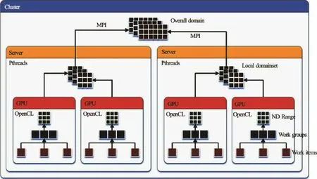
Fig.2 Representation of the three synchronization and parallelization levels present within the HiPIMS MPI software

The underlying system drivers manage the vectorization for low-level optimization, and deployment of this code on the hardware available, which need not be limited to GPUs but could also include hybrid-style processors (APUs), or IBM cell processors. Data is transferred to the device’s own DRAM memory before computation begins, and transferred back as infrequently as possible, allowing for status updates and filebased storage of results. Transferring both instructions and large volumes of data across the host bus is far from desirable, and would represent a major bottleneck in the process if undertaken too frequently. However, as the total domain size increases, the delay introduced by latency across the host bus, as a proportion of overall computation time, becomes a diminishing portion. This presents an opportunity for domain decomposition, but only for instances where the problem size is sufficient to justify frequent data transfer.

Achieving parallelism across multiple devices in a single computer system becomes more difficult, for which domain decomposition is required. Achieving a numerically sound solution in either sub-domain remains dependent on neighboring cells, and thus data must be transferred between the two or more computational devices involved. Owing to the speed constraints of the host bus, these exchanges are computationally expensive, and so to reduce the frequency required we need not exchange data after every time step, provided there is a sizeable overlap between the two sub-domains. By merit of the CFL condition, any error arising in the solution at the extremities of the domain, because neighbor data lacks currency, will only propagate by one cell at a time. This allows these errors to be corrected, providing the overlap is notspent by the time data is exchanged between compute devices. In the event overlap is exhausted, a rollback to the last saved state is required (see Fig.1). This is nonetheless dependent on the maximum time step being calculated after each iteration, making some host bus transfers inevitable but minimizing their size. The requirement for an overlap also means a model must consist many millions of cells before decomposition to multiple devices becomes a worthwhile pursuit. A separate CPU thread is used to manage each compute device, accepting some idle resource for a short period of time, for example in a tidal inundation model an entire sub-domain could be dry before the wave arrives.

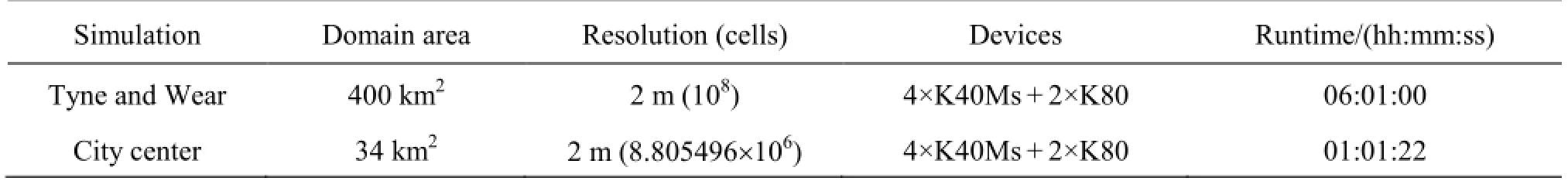
Table 1 HiPIMS performance for the Newcastle flood simulations

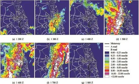
Fig.3 Rainfall radar centered on Newcastle upon Tyne for the 28 June 2012 event

A further extension to this approach, allowing further compute devices to be engaged residing in different physical computer systems, is achieved through MPI (see Fig.2). Cell data is exchanged over high-speed network connections, and only directed to the systems which require it. Reduction to identify the next timestep is undertaken locally on a compute device, then across all local devices, and finally by broadcast messages between all MPI nodes. Three levels of synchronization exist encompassing the device, system, and all systems.

3. Application and model performance

With HiPIMS, we demonstrate that high-resolution large-scale flood inundation modeling can be realized at an affordable computational cost through an application to reproduce the June 2012 Newcastle flood event. During a few hours, rainfall intensities in excess of 200 mm/h were recorded, and in excess of 50 mm of rainfall caused chaos across the city. The event caused widespread disruption as a consequence of timing coincident with peak travel times for commuters. Arterial road, rail and public transport services were all disrupted or suspended during the incident.

Two simulations have been carried out with a 2 m resolution, one covering 36 km2of Newcastle central area and another covering 400 km2of Tyne and Wear, which respectively involve 8×106and 108computational cells. Due to the flashy nature of the flood event, no organized field measurements are available for model validation. Crowd-sourced data (including pictures and videos from the public and messages from online social networks) were collectedand used to verify model results. The runtimes of the two simulations are presented in Table 1, confirming the model performance. Real-time or faster prediction is achieved for both simulations, demonstrating the potential of HiPIMS for wider applications in flood forecasting and risk management.

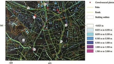
Fig.4 Extract of flood depths for the center of Newcastle upon Tyne

Domain inputs used for all simulations were extracted from UK Met Office C-band rainfall radar (NIMROD) from 12:00 UTC to 18:00 on 28 June 2012, shown in Fig.3. The Tyne and Wear model covers the full extent with highest rainfall totals, for the flood event considered as per rainfall radar. Specifically, this spans from (4.15×105, 5.55×105) to (4.35× 105, 5.75×105) on the British National Grid (OSGB36). Bed elevations are in effect a digital elevation model, obtained by superimposing buildings from the firstpass return of an Environment Agency LiDAR survey atop a filtered terrain model, blended with OS Terrain 5 data where LiDAR coverage was lacking. This produces an elevation model where buildings are present, as important in determining the direction of flow, but vegetation which would provide minimal flow resistance (e.g. trees and bushes) are omitted. Buildings are not superimposed in the case of bridges and similar overhead structures, where a viable flow pathway is likely to exist beneath. Whilst imperfect insofar as there may be locations where flow could exist on two different levels within the same location, this is considered to be a practical compromise. Generation of the elevation model was automated by processing OS MasterMap Topography Layer data to identify building outlines and overhead structures. A Manning coefficient of 0.2 is used across the whole domain, sensitivity studies suggest minimal effect on flood depths for this model. Cells which would ordinarily contain water, including ponds and rivers, were disabled from computation to allow the simulation to focus entirely on pluvial flooding processes.

Following the flood event, members of the public were invited to contribute photos and their respective locations for flooding through a dedicated website, which was advertised across the region using local television and radio. Social media activity from Twitter was also archived for analysis, more information on which can be found in Smith et al.[25]. The locations of a handful of photos alongside simulation results for the maximum depths are shown in Fig.4, where it is clear there is a strong agreement between the locations of the crowd-sourced photos and flooding. On the A167(M) Central Motorway, at points A and F it can be seen that dips in the road for intersections have suffered from serious flooding, which is an unfortunate consequence of the transport infrastructure design in Newcastle, and reinforces that some settlements are more exposed to the risk of pluvial flooding. Some of the longest overland flow pathways converge at point C on the Newcastle University campus, and G near The Gate entertainment complex, and these are clearly visible as some of the highest depths. Points E and D highlight some of the limitations of the approach, with the football pitch at E seeing exaggerated flooding because infiltration and drainage is not adequately represented, and a large pool appearing at D where in fact the railway line goes underground, but topographic data obtained did not reflect this. Point B represents a pedestrian passageway under a major road, which is accurately represented and was known to flood, however the road above is not represented and was also flooded. As a whole, the simulation results provide an accurate representation of the floodingwhich occurred in June 2012, albeit with scope for improvements by manual intervention in a handful of places.

Fig.5 Sample areas of interest from the model results, showing (a) Checkerboard effect with coarse DTM source data, (b) Exaggerated depths above a large drainage culvert, (c) Flooding predicted around underpasses, (d) Complex network of underpasses and road tunnels, (e) Railway tunnel not represented properly, and (f) Sacrificial land area

Examining the results for the model domain as a whole, some specific areas of interest have been extracted and are shown in Fig.5. Whilst resampled 5 m DTM data provides a basis for ensuring flow connectivity in areas where 2 m LiDAR coverage was lacking, the results in the 5 m areas are not satisfactory. The checkerboarding effect shown in Fig.5(a) is a consequence of the inferior numerical resolution of the 5 m DTM data and resampling algorithm. Increased LiDAR coverage remains essential to improving our understanding of surface water flood risk. The flooding shown in Fig.5(b) is exaggerated slightly, this area is underlain by a large culverted watercourse now used as a sewer, which is not adequately represented by the drainage assumptions made uniformly across the domain. It is important to note that even with more information, accurately predicting the capacity of this long-culverted watercourse would prove difficult. Flooding in pedestrian underpasses is a known issue in Newcastle upon Tyne, while they are not necessarily captured by the single-level DEM used by the model, in many cases the entrances to the underpasses are sunk and therefore capture risk, such as shown in Fig.5(c) but not as well represented for a more complex network of underpasses, tunnels and roads shown in Fig.5(d). Accurate data for the railway network in the UK, including the alignment of tunnels, was not available and hence the backwater shown in Fig.5(e) is an erroneous artefact of a railway tunnel under a number of buildings. The area shown in Fig.5(f) did flood, but not to the extent shown, this is a basin used as sacrificial land, with a children’s playground for use during normal conditions. The uniform drainage assumptions have underestimated the capacity of the soil infiltration in this area.

4. Conclusions

Presented in the context of flooding, this work demonstrates the great potential of high-performance heterogeneous computing techniques in advancing the field of computational hydraulics. Using the High-Performance Integrated Modelling System (HiPIMS) that supports shock-capturing hydrodynamic simulation of shallow flows across multiple GPUs and multiple systems, a city-scale urban flood event induced by intense rainfall was reproduced at a very high resolution (2 m cell size, 108computational nodes). This may indicates a new era for the development of computational hydraulics, in which complex hydrodynamic models can now be applied to support regional/catchment-scale high-resolution simulations in real-time, providing a revolutionary tool/technology for implementing the new generation of natural hazard forecasting and risk management strategies.

Remaining challenges have been considered, such as the need for greater ubiquity of LiDAR coverage not just limited to urban areas, but their upstream catchments, and the issues surrounding our limited knowledge of long-culverted watercourses and aging drainage network, or antecedent conditions affecting infiltration capacity. Nonetheless the model results are a good match against crowd-sourced information from an event on 28 June 2012, despite a few notable areas where improvements could be made. Computational performance itself should not be considered a limiting factor in hydraulic modelling, as software capable of leveraging heterogeneous and large distributed computer systems becomes increasingly widespread.

Acknowledgement

This work was supported by the UK Natural Environment Research Council (NERC) SINATRA project (Grant No. NE/K008781/1).

[1] Bates P. D., De Roo A. P. J. A simple raster-based model for flood inundation simulation [J]. Journal of Hydrology, 2000, 236(1-2): 54-77.

[2] Bradbrook K. F., Lane S. N., Waller S. G. et al. Two dimensional diffusion wave modelling of flood inundation using a simplified channel representation [J]. International Journal of River Basin Management, 2004, 2(3): 2111-223.

[3] Yu D., Lane S. N. Urban fluvial flood modelling using a two-dimensional diffusion-wave treatment, Part 1: Mesh resolution effects [J]. Hydrological Processes, 2006, 20(7): 1541-1565.

[4] Costabile P., Costanzo C., Macchione F. Comparative analysis of overland flow models using finite volume schemes [J]. Journal of Hydroinformatics, 2011, 14(1): 122-135.

[5] Fewtrell T. J., Neal J. C., Bates P. D. et al. Geometric and structural river channel complexity and the prediction of urban inundation [J]. Hydrological Processes, 2011, 25(20): 3173-3186.

[6] Hunter N. M., Bates P. D., Néelz S. et al. Benchmarking 2D hydraulic models for urban flooding [J]. ICE-Water Management, 2008, 161(1): 13-30.

[7] Wang Y., Liang Q., Kesserwani G. et al. A positivity-preserving zero-inertia model for flood simulation [J]. Computers and Fluids, 2011, 46(1): 505-511.

[8] Liang Q., Du G., Hall J. W. Flood inundation modelling with an adaptive quadtree shallow water equation solver [J]. Journal of Hydraulic Engineering, ASCE, 2008. 134(11): 1603-1610.

[9] George D. L. Adaptive finite volume methods with wellbalanced Riemann solvers for modeling floods in rugged terrain: Application to the Malpasset dam-break flood (France, 1959) [J]. International Journal for Numerical Methods in Fluids, 2011, 66(8): 1000-1018.

[10] Soares-Frazão S., Lhomme J., Guinot V. et al. Twodimensional shallow-water model with porosity for urban flood modeling [J]. Journal of Hydraulic Research, 2008, 46(1): 45-64.

[11] Chen A. S., Evans B., Djordjevića S. et al. Multi-layered coarse grid modelling in 2D urban flood simulations [J]. Journal of Hydrology, 2012, 470-471: 1-11.

[12] Neal J. C., Fewtrell T. J., Bates P. D. A comparison of three parallelisation methods for 2D flood inundation mode-ls [J]. Environmental Modelling and Software, 2010, 25(4): 398-411.

[13] Sanders B. F., Schubert J. E., Detwiler R. L. ParBreZo: A parallel, unstructured grid, Godunov-type, shallow-water code for high-resolution flood inundation modeling at the regional scale [J]. Advances in Water Resources, 2010, 33(12): 1456-67.

[14] Lamb R., Crossley M., Waller S. A fast two-dimensional floodplain inundation model [J]. ICE-Water Management, 2009, 162(6): 363-370.

[15] Kalyanapu A. J., Shankar S., Pardyjak E. R. et al. Assessment of GPU computational enhancement to a 2D flood model [J]. Environmental Modelling and Software, 2011, 26(8): 1009-1016.

[16] Brodtkorb A. R., Sætra M. L., Altinakar M. Efficient shallow water simulations on GPUs: Implementation, visualization, verification, and validation [J]. Computers and Fluids, 2012, 55(4): 1-12.

[17] Néelz S., Pender G. Benchmarking the latest generation of 2D hydraulic modelling packages [M]. Bristol, UK: Environment Agency, 2013.

[18] Smith L. S., Liang Q. Towards a generalised GPU/CPU shallow-flow modelling tool [J]. Computers and Fluids, 2013, 88(12): 334-343.

[19] Sætra M. L., Brodtkorb A. R. Shallow water simulations on multiple GPUs [J]. Applied Parallel and Scientific Computing, 2012, 7134: 55-66.

[20] Jin S. Asymptotic preserving (AP) schemes for multiscale kinetic and hyperbolic equations: A review [J]. Rivista di Matematica della Università di Parma, 2012, 2(2): 177-216.

[21] Xia X., Liang Q., Ming X. et al. An efficient and stable hydrodynamic model with novel source term discretisation for overland flow simulations [J]. Water Resources Research, 2016 (under review).

[22] Audusse E., Bouchut F., Bristeau M.-O. et al. A fast and stable well-balanced scheme with hydrostatic reconstruction for shallow water flows [J]. SIAM Journal on Scientific Computing, 2004, 25(6): 2050-2065.

[23] Liang Q., Borthwick A. G. L. Adaptive quadtree simulation of shallow flows with wet-dry fronts over complex topography [J]. Computers and Fluids, 2009, 38(2): 221-234.

[24] Smith L. S., Liang Q., Quinn P. F. Towards a hydrodynamic modelling framework appropriate for applications in urban flood assessment and mitigation using heterogeneous computing [J]. Urban Water Journal, 2015, 12(1): 67-78.

[25] Smith L. S., Liang Q., James P. Assessing the utility of social media as a data source for flood risk management using a real-time modelling framework [J]. Journal of Flood Risk Management, 2015, doi:10.1111/jfr3.12154.

(Received June 11, 2016, Revised October 16, 2016)

* Project supported by the UK NERC SINATRA Project (Grant No. NE/K008781/1).

Biography:Qiuhua LIANG (1974-), Male, Ph. D., Professor