Water medium retarders for heavy-duty vehicles: Computational fluid dynamics and experimental analysis of filling ratio control method ＊

Hong-peng Zheng (郑宏鹏), Yu-long Lei (雷雨龙), Peng-xiang Song (宋鹏翔)

State Key Laboratory of Automotive Simulation and Control, College of Automotive Engineering, Jilin University,Changchun 130022, China, E-mail:zhenghp13@mails.jlu.edu.cn

Introduction

With the development of the road transport industry, the load of the vehicles and the distance to the destination are increased. A heavy-duty vehicle(HDV) is a mass dominant system and a braking torque is frequentlyrequired to regulate the vehicle velocity because of the road complexity. If only theservice brake is involved under the braking conditions, high kinetic energy of the vehicle willtotally be converted to the thermal energy of the brake shoe. The brake shoe might suffer from the heat recession caused by the high temperature in its long-term usage,tosignificantly reduce the braking capacity and to threat the road safety[1-3].

In view of the braking problem stated above,abraking system is adopted by the HDVs to produce the braking torque as required. The braking system[4]includes the engine brake, the hydraulic retarder brake and the service brake. The engine brake[5]has afixed braking torque once activated and could not be regulated according to the braking requirements.However, the braking torque of the hydraulic retarder[6]could be adjusted according to the needs.When a vehicle is driven under non-emergency braking conditions, its braking system could control the engine brake and the hydraulic retarder brake to produce a braking torque to satisfy the braking requirements without using the service brake[4], thus, the time and the frequency of using the service brake are reduced. This control scheme can protect the service brake from the heat recession and to better use itsbraking capacity under emergency braking conditions[6,7].

The hydraulic retarder could produce a braking torque by converting the kinetic energy of the vehicle to the thermal energy of the working fluid[8,9]. The novel hydraulic retarder is a water medium (WM)retarder, and the working fluid is the coolant from the coolant circulation. The heat produced along with the braking torque can be dissipated by a radiator in the coolant circulation[10]. The WM retarder should produce a controllable braking torque to satisfy the braking requirement sunder complex braking conditions and then the time and the frequency of the service brake usage can be greatly reduced[11,12]. The braking torque of the WM retarder can be adjusted by the filling ratio[13](the volume ratio between the fluid and the air) of the working chamber when the vehicle velocity is constant. The flow field of the working chamber was extensively studied by using the computational fluid dynamics (CFD), including the influence of the diameter of the circulation circle, the number and the angle of the blade on the braking torque of the hydraulic retarder and the corresponding flow field[14], and the flow distribution when the working chamber is partly filled with working fluid based on the two-phase flow[15]. However the mechanism of the generation of the braking torque and the key factors that could influence the filling ratio are not clearly revealed, and the control strategy of the WM retarder remains an issue to explore.

This paper introduces the coolant circulation and the construction of the WM retarder. The flow distribution is analyzed by using the fluid mechanics.The mechanism of the generation of the braking torque is expressed mathematically and the key factors that could influence the filling ratio and the braking torque are analyzed, which could be directly used in analyzing the control strategy of the WM retarder.CFD simulations are conducted to compute the braking torque by using the Reynolds averaged Navier-Stokes (RANS) and shear stress transport(SST) turbulent models, respectively. Experiments are conducted to verify the CFD simulation results and justify the key factors proposed in this study. Finally,the flow field of the working chamber is examined to analyze the character of the flow distribution.

1. Basic analysis of the hydraulic retarder

1.1 Coolant circulation

Figure 1(a) shows the working mode of the coolant circulation system when a WM retarder is not activated. The coolant is pumped into the engine water jacket from the pump to cool down the engine. The two-position, three-way control valve is then closed,allowing the coolant to directly flow into the thermostat and to decide whether to flow into the radiator according to the temperature setting. This circulation system is similar to a traditional engine coolant circulation system. The working mode of the coolant circulation system when a WM retarder is activated is illustrated in Fig.1(b). In this mode, the two-position,three-way control valve is opened, compelling the coolant to directly flow from the engine water jacket to the WM retarder. Subsequently, the coolant flows into the thermostat in a similar manner as when a WM retarder is not activated.

1.2 Construction analysis

The principal part of the WM retarder consists of the sealing component, the rotor, and the stator, as shown in Fig.2. The working chamber is formed by the rotor and the stator, and the sealing component is used to seal the working chamber. The sealing component is fixed on the stator by bolts, and the stator is fixed to the vehicle. The rotor is connected to the drive shaft by a spline. When the vehicle is being driven, the rotor rotates with the drive shaft constantly.

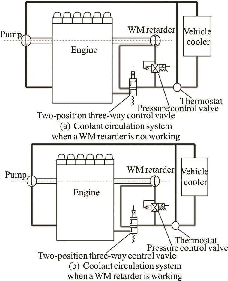
Fig.1 Sketches of the cooling circulation with WM retarder

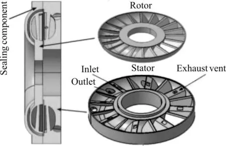
Fig.2 Sketch of the WM retarder

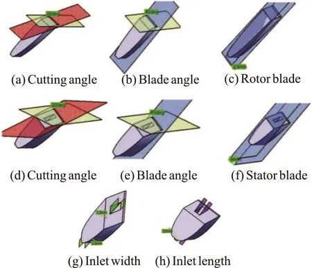
Fig.3 (Color online) Sketch of the circulation circle and the blades

When a braking torque is required, the coolant flows into the working chamber through the inlet on the stator. Meanwhile, the air in the working chamber flows out through the exhaust vent on the stator. The coolant continuously generates a braking torque with the rotating rotor and then flows out of the working chamber through the outlet on the stator. In the process, the WM retarder converts the kinetic energy of the vehicle to the thermal energy of the coolant.The dimension information of the circulation circle and the blades are shown in Table 1 and Fig.3.

Table 1 Parameters of the hydraulic retarder

1.3 Mathematical model

When the WM retarder is working, the rotor can produce a braking torque. This section focuses on the force analysis of the mean flow in the working chamber through fluid mechanics. The generation of the braking torque is analyzed. The fluid domain of the working chamber is shown in Fig.4.

Fig.4 The flow direction of the mean flow in the working chamber

The rotational direction is shown in Fig.4. In a working circulation, the working fluid flows from position 1 to position 2 because of the centrifugal force of the rotational rotor. It flows to the stator from position 2 to position 3, and from position 3 to position 4 because of the inertial force before finally it flows to the rotor from position 4 to position 1.

Fig.5 Working circulation in the working chamber

The braking torque produced by the WM retarder should be analyzed in the rotor domain depicted in Fig.5. The fluid domain and the solid object of the rotor are taken as the control volume. The interface between the rotor and the stator is takenas the control surface. The resultant force1F is generated when the working fluid flows from position 11()v to position 22()v . By analyzing the fluid mechanics, the linear momentum equation of this process can be expressed as[16]

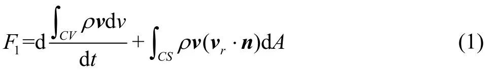
where1F is the resultant force along the direction of the fluid velocity, vis the fluid velocity,rvis the fluid velocity relative to the control surface, n is the direction normal to the control surface.

The flow field in the WM retarder is unsteady.However, the concern of this paper is the overall flow field, therefore, it is not important how the flow is developed. The working fluid in this research is incompressible, and Eq.(2) can be simplified as

For a fixed control volume

Equation (1) then becomes

where m˙ is the working flow rate into and out of the rotor,avgv is the average velocity of the working fluid into and out of the rotor and ρ is the density of the working fluid[13].

In Fig.6,1csA is the area where the working fluid flows into the rotor by the inertial force.2csA is the area where the working fluid flows out of the rotor by the centrifugal force. The areas of1csA and2csA are equal because of the conservation of mass.

We can infer that

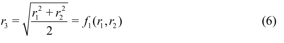
Fig.6 (Color online) Interface of the rotor

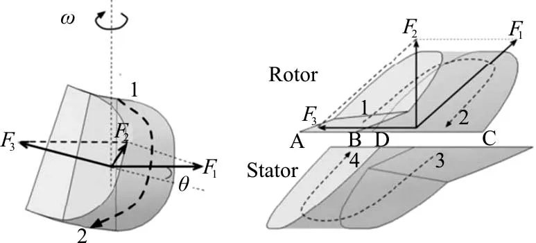
Fig.7 Force analysis of the rotor

The force analysis of the rotor is shown in Fig.7.where θ is the angle of the blades and3F is the component of the resultant force, normal to3r in the interface of the rotor.3F and3r form the braking torque.2F is the component of the resultant force,normal to the interface of the rotor.

From Eqs.(2), (3) and (4), the braking torque of the hydraulic retarder is

From the Buckingham Theory[11], it can be inferred that

where k and j are the coefficients, α is the filling ratio and1f,2f,3f are the functions of the diameter of the circulation circle.

1.4 Filling ratio control method

The outlet of the working chamber is located at position 3 in Fig.4. When the fluid flows to position 3,the kinetic energy is increased with the rotational speed, causing the pressurewcP at the outlet to be large and closelyrelated with the rotational speed and the filling ratio of the working chamber.

The Refs.[14,15] support the flow distribution generated by the CFD simulations. The flow distribution can be summarized as follows:

(1) The outlet pressureincreases with the filling ratio while the rotational speed of the rotor remains constant.

(2) The outlet pressureincreases with the rotational speed while the filling ratio of the working chamber remains constant.

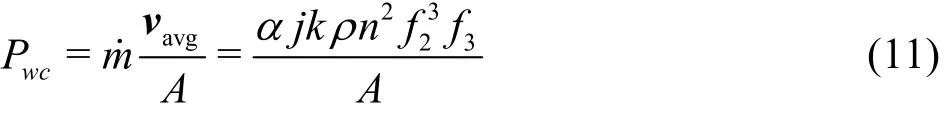
Through a fluid mechanics analysis, the relationships among the rotational speed, the outlet pressure,and the filling ratio can be expressed as[16]

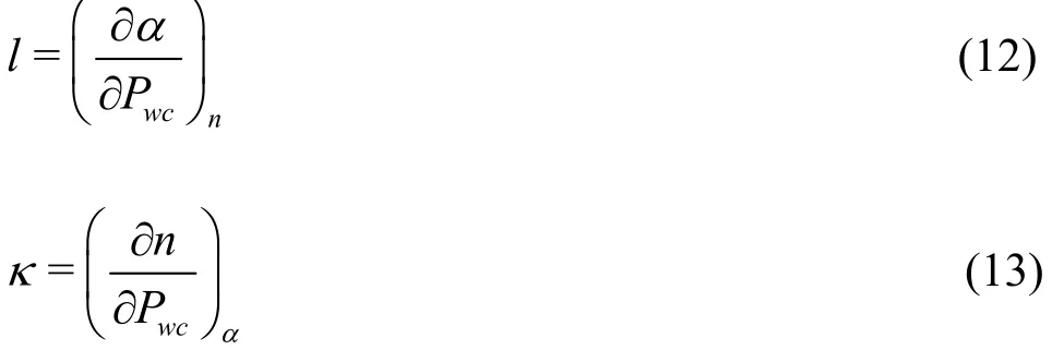
where l is the coefficient of the filling ratio, κ is the coefficient of the rotational speed,wcP is the pressure at the outlet of the working chamber, and n is the rotational speed of the rotor.

A large value of l indicates that a large change of the filling ratio is needed to cause a small fractional change of the pressureat the outlet of the working chamber while the rotational speed of the rotor remains constant. A large value of κ indicates that a large change of the rotational speed of the rotor is needed to cause a small fractional change of the pressurewcP at the outlet of the working chamber while the filling ratio of the working chamber remains constant. The WM retarders of different dimensions have different l and κ values.

In conclusion, when a specific filling ratio is required, the pressure control valve mounted at the downstream of the outlet can control the outlet pressure by simply increasing or decreasing the outlet pressure to make it equal to the target pressure, and the specific filling ratio of the working chamber can be automatically determined by Eq.(9) and (10).

2. CFD simulations and experimental verification

2.1 Numerical method

This section focuses on the CFD simulations ofthe working chamber. The simulations are performed by using the ANSYS CFX solver, which is based on a three-dimensional incompressible finite-volume method. The temperature increase should be analyzed because of the conversion of the mechanical energy of the vehicle to the internal energy of the working fluid.The energy conversion is important in this case, and the energy equation must be solved simultaneously.The mean flow and the effects of the turbulence on the mean flow properties are emphasized in this section as well. The RANS and SST are used as the turbulent models in the CFD simulations. A high-resolution scheme with a second-order accuracy is used for the discretization[17,18]. Figure 8 depicts the computational domain, including the working chamber, the total inlet,and the outlet region. The working chamber includes the rotor domain, the stator domain, and the connection domain. The unstructured grid is generated by using the ANSYS mesh program. The meshes are optimized for different parts, and the optimization parameters are listed in Table 2. The focus is on how a steady status is achieved and not so much on how a flow is established; therefore, a steady analysis is performed. The parameters of the working fluid are listed in Table 3, and the boundary conditions are listed in Table 4.

Table 2 Parameters of the mesh optimization

Table 3 Parameters of the working fluid

Table 4 Boundary conditions of the CFD simulations

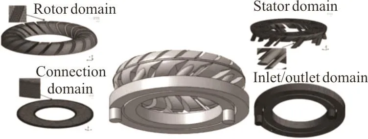
Fig.8 Mesh optimization of the computational domain

A grid independence analysis is performed to avoid the errors owing to the coarseness of a grid, and the numbers of intervals are increased by 20% in all directions. The CFD simulations are stabilized until the braking torque fluctuates within 0.3% of the torque monitor[19]. Figure 9 presents a comparison of the results of simulations using coarse, medium, and fine grids, with the RANS and SST as the turbulent models.The x-coordinate (RS) represent rotational speed of the rotor and the y-coordinate (BI) represent the braking torque. The error analysis indicates that the fine grid provides a satisfactory resolution for the RANS and the SST. The error between the two turbulent models is small when the rotational speed of the rotor is small, and the error increases with the rotational speed of the rotor.

Fig.9 Grid independence analysis

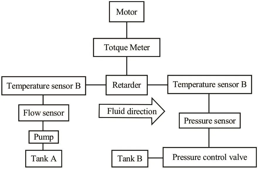
Fig.10 Schematic diagram of the test bed

2.2 Experimental procedure

A test bed is built (Fig.10) to analyze the braking performance of a WM retarder[20]. The specifications and the uncertainties of the measurement devices are shown in Table 5. The experiments include three steps.

Table 5 Specifications and uncertainties of the measure- ment devices

Step 1: The motor is activated. The rotational speed of the rotor is adjusted to 1 200 rpm. The mass flow rate of the pump is adjusted to 180 L/min.

Step 2: The outlet pressure control valve is adjusted from the maximum opening to the minimum opening to maintain the value of the pressure sensor(Pop) within that listed in Table 5. The values generated by the torque meter and the temperature sensor B are recorded.

Step 3: Steps 1 and 2 are repeated with the rotational speed set to 1 500 rpm and then to 1 800 rpm.

2.3 Result verification

Figure 11 shows the comparison between the results of the CFD simulations and the experiments.The x-coordinate represent outlet pressure and the y-coordinate represent the braking torque. Figure 11(a) and Fig.11(b) show that the CFD simulation by using the SST turbulent model is more accurate than that by using the RANS turbulent model, and the errors are within 5%. Figure 11(a) shows the braking torque at different outlet pressures. When the rotational speed is held constant, the outlet pressure can be increased by reducing the outlet channel, the pressure of the working chamber can be determined by the outlet pressure, and then the braking torque increases with the outlet pressure. Figure 11(b) shows the temperature rising at different outlet pressures.When the braking power increases, an increasing amount of the kinetic energy is converted to the thermal energy, and the temperature of the coolant increases, as detected at the outlet.

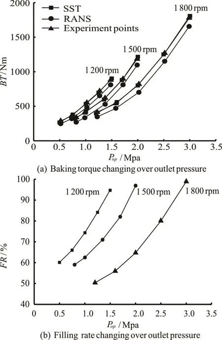
Fig.11 Comparison between CFD simulation and experimental results

Figure 12(a) shows the computational results of the outlet pressure against the filling rate while the rotational speed remains constant. The x-coordinate represent outlet pressure and the y-coordinate represent the temperature rise of the working fluid and the filling rate (FR) of the working chamber,respectively. From Fig.12(a), a higher outlet pressure is needed to keep the same filling rate of the working chamber when the rotational speed is increased.Figure 12(b) shows the fluid volume fractions in the rotor and the stator. When the flow in the working chamber is stable, the volume fractions of the rotor and the stator are supposed to be the same because the rotor and the stator are in symmetric positions.However, the fluid volume fraction in the stator is larger than that in the rotor domain. This result is due to the mounting of the inlet and the outlet on the stator domain and the filling of both with coolant without air.

The engine drives the pump in the HDV coolant circulation system, thus, the mass flow rate of the coolant is determined by the rotational speed of the engine. When the vehicle is being driven on the road,the mass flow rate of the coolant circulation system is dynamically changed. Figure 13 shows the comparison between the CFD simulation and the experimental results against the braking torque with respect to the outlet pressure when the mass flow rate varies. The results show that the mass flow rate does not influence the braking torque. In conclusion, the braking torque is totally determined by the rotational speed and the filling ratio, which is controlled only by the outlet pressure.

Fig.12 CFD simulation results

Fig.13 Braking torques for different mass flow rates

2.4 Flow distribution analysis

Figure 14(a) shows the positions of the analytic planes. Figure 14(b) shows the flow distributions in the planes when the rotational speed is 1 500 rpm. The red area represents the coolant, whereas the blue area represents the air. Rows X, Y and Z show the flow distributions when the filling ratios are 92.9%,73.3%, and 58.5%, respectively. In row X, the fluid volume fraction is 92.9%, and the amount of air is relatively small. The flow distribution in the plane mainly reflects the red region. However in row Z,the air volume fraction increases, and the flow distribution reflects a large blue region. The flow distributions represented in column A, Row Y and column E, row Y show that the fluid is mainly concentrated outside the circulation circle because of the centrifugal force and the inertial force caused by the rotational rotor. Moreover, the air is distributed at the center of the circulation circle. The flow distributions represented in column A, row Z and column B, row Z show that the coolant is mainly concentrated on the pressure side of the blades and that the air is concentrated on the suction side of the blades because of the centrifugal force and the inertial force.

Fig.14 (Color online) Flow distribution analysis for partly filled cases

3. Conclusions

This paper presents the construction of a WM retarder and the coolant circulation system when a WM retarder is involved. On the basis of the mathematical model of a WM retarder, the filling ratio control method is analyzed. The CFD simulations are carried out by using RANS and SST turbulent models.Experiments are conducted to verify the CFD simulation results and justify the control method proposed in this study. Compared with the experimental results,the results of the CFD simulation by using the SST turbulent model is more accurate than those obtained by using the RANS turbulent model. The results also show that the control method obtained by the CFD and fluid mechanics analysis in this paper can effectively control the filling ratio of the WM retarder.Finally, the flow field of the working chamber is examined to analyze the character of the flow distribution. Several conclusions are as follows:

(1) The filling ratio of the WM retarder is determined by the rotational speed of the rotor and the outlet pressure but is not influenced by the mass flow rate into and out of the working chamber.

(2) The braking torque of the hydraulic retarder,when the model is confirmed, is determined by Eqs.(5)-(7), which indicates that the blades angle, the working fluid rate into and out of the rotor and the average velocity of the working fluid are the key parameters. To maximize the braking torque, the desirable blade angle should be selected with aspecific model and the smooth circulation circle should be preferred to increase the mass flow rate and the average velocity of the working fluid.

(3) The fluid is mainly concentrated outside the circulation circle and on the pressure side of the blades because of the centrifugal force and the inertial force. The air is mainly concentrated at the center of the circulation and on the suction side of the blades.The outlet for the air should be located at the center of the circulation, where the air is concentrated.

(4) In the analysis of the control strategy of the WM retarder, the relationships among the rotational speed, the outlet pressure, and the filling ratio can be obtained by CFD simulations. The relationship between the position of the spool of the valve and the outlet pressure can be obtained by experiments. Then,the braking torque can be controlled by controlling the outlet pressure of the WM retarder, and the braking requirements can consequently be satisfied.

(5) The SST turbulent model is more accurate in the CFD simulation, especially in the simulations of the rotational flows, as is verified in this research. The braking torque temperature rise errors between the CFD and the experiments are within 5%.

Acknowledgements

This work was supported by the Program for New Century Excellent Talents in University (Grant No. NCET-08-0248), the 985 Project Automotive Engineering of Jilin University.

[1] Gigan G., Vernersson T., Lundén R. et al. Disc brakes for heavy vehicles: An experimental study of temperatures and cracks [J]. Proceedings of the Institution of Mechanical Engineers, Part D: Journal of Automobile Engineering, 2015, 229(6): 684-707.

[2] Tretsiak D. Experimental investigation of the brake system’s efficiency for commercial vehicles equipped with disc brakes [J]. Proceedings of the Institution of Mechanical Engineers, Part D: Journal of Automobile Engineering,2012, 226(6): 725-739.

[3] Yuan Z., Ma W., Liu C. et al. Temperature field analysis of the open-type hydrodynamic retarder of heavy vehicle[J]. Journal of Jilin University (Engineering and Technology Edition), 2013,43(5): 1271-1275(in Chinese).

[4] Liu Z., Zheng H., Xu W. et al. A downhill brake strategy focusing on temperature and wear loss control of brake systems [R]. SAE Technical Paper 2013-01-2372, 2013.

[5] Jia P., Xin Q. H. Compression-release engine brake modeling and braking performance simulation [J]. SAE International Journal of Commercial Vehicles, 2012 , 5(2) :505-514.

[6] Zheng H., Lei Y., Song P. Designing the main controller of auxiliary braking systems for heavy-duty vehicles in nonemergency braking conditions [J]. Proceedings of the Institution of Mechanical Engineers, Part C: Journal of Mechanical Engineering Science, 2017,0954406217706386.

[7] Cho H. J., Cho C. D. A study of thermal and mechanical behaviour for the optimal design of automotive disc brakes [J]. Proceedings of the Institution of Mechanical Engineers, Part D: Journal of Automobile Engineering,2008, 222(6): 895-915.

[8] Zheng H., Lei Y., Song P. Design of a filling ratio observer for a hydraulic retarder: An analysis of vehicle thermal management and dynamic braking system [J].Advances in Mechanical Engineering, 2016, 8(10):1687814016674098.

[9] Lei Y., Song P., Zheng H. et al. Application of fuzzy logic in constant speed control of hydraulic retarder [J].Advances in Mechanical Engineering, 2017, 9(2):1687814017690956.

[10] Zheng H., Lei Y., Song P. Design of the filling-rate controller for water medium retarders on the basis of coolant circulation [J]. Proceedings of the Institution of Mechanical Engineers, Part D: Journal of Automobile Engineering, 2016, 230(9): 1286-1296.

[11] Li J., Cai Z., Jia Z. Simulation of constant speed control on coach hydraulic retarder on special weather condition [J].Journal of System Simulation, 2014, 26(11): 2765-2769.

[12] Lu X. Y., Hedrick J. K. Heavy-duty vehicle modelling and longitudinal control [J]. Vehicle System Dynamics, 2005,43(9): 653-669.

[13] Li X., Cheng X., Miao L. Large eddy simulation on internal flow field of hydraulic retarder and characteristics prediction [J]. Journal of Central South University(Science and Technology), 2012: 43(5): 1718-1723(in Chinese).

[14] Lu X.,Wu Y., Ma X. et al. Dynamic flow simulation and performance prediction of torque limited hydrodynamic coupling [J]. Huazhong University of Science and Technology (Natural Science Edition), 2015, 43(2):27-29(in Chinese).

[15] Rao Y., Li C., Huang J. Study on two-way FSI of hydraulic retarder [J]. Machine Tool and Hydraulic, 2015,43(1): 117-122(in Chinese).

[16] Yunus A. C., Cimbala J. M. Fluid mechanics: Fundamentals and applications [M]. International Edition, New York, USA: McGraw Hill Publication, 2006, 185-201.

[17] Zhou S. J., Tian M. C., Zhao Y. E. et al. Dynamic modeling of thermal conditions for hot-water districtheating networks [J]. Journal of Hydrodynamics, 2014,26(4): 531-537.

[18] Li D. H., Xu J. Y. Measurement of oil-water flow via the correlation of turbine flow meter, gamma ray densitometry and drift-flux model [J]. Journal of Hydrodynamics, 2015,27(4): 548-555.

[19] Zhang W., Ma Z., Yu Y. C. et al. Applied new rotation correction k-ω SST model for turbulence simulation of centrifugal impeller in the rotating frame of reference [J].Journal of Hydrodynamics, 2010, 22(5): 404-407.

[20] American National Standard. engine retarder dynamometer test and capability rating procedure [R]. SAE Technical Standard, 1994.