Two timescales for longitudinal dispersion in a laminar open-channel flow ＊

Yu-fei Wang (王宇飞), Wen-xin Huai (槐文信), Zhong-hua Yang (杨中华), Bin Ji (季斌)

State Key Laboratory of Water Resources and Hydropower Engineering Science,WuhanUniversity,Wuhan 430072, China, E-mail: yufeiwang@whu.edu.cn

The longitudinal dispersion is an important issue in studying the scalar transport in flow systems (e.g.,the open-channel flow and the pipe flow)[1,2]. The longitudinal dispersions share the same behavior although the cross sections of the flow systems may be different (e.g., rectangular and circular sections),thus it is helpful to study the longitudinal dispersion in the laminar open-channel flow. When the time scale is large, the longitudinal dispersion coefficient, which reflects the spreading rate in the longitudinal direction,can be solved easily. Using some reasonable assumptions (e.g., the longitudinal diffusion can be omitted when the Peclet number ( )Pe is large), Chatwin and Sullivan[1]found that the dispersion coefficient for the laminar channel flow can be expressed as =kis the mean velocity andzD the transverse diffusion coefficient. However, the formula given by Chatwin and Sullivan[1]can only be used at a large timescale when the transverse concentration distribution is uniform and the longitudinal concentration is in a Gaussian distribution. This is because in the early stage, the actual problems are as follows: (1) the transverse concentration distribution is nonuniform, (2)the longitudinal dispersion coefficient is not a constant value and (3) the longitudinal mean transverse concentration is not in a Gaussian distribution, with absolutethe thn integral central moment of c

wheregx is the location of the centre of gravity. Thus,the initial stage of the scalar transport was widely studied[3-5]. However, the timescales vary from one study to another, and without experiments to verifytheir results due to the demanding experimental conditions. One might be confused in the face of many conflict results. Therefore, the study of the dimensionless timescales could offer an alternative simple stan-dard to evaluate the previous theoretical studies.

In this letter, we concentrate on the developments of the transverse uniformity index ( )UI, the dimen- sionless history mean longitudinal dispersion coeffi- cient ()K , the dimensionless temporal longitudinal dispersion coefficient (Kt) and the absolute skewness of longitudinal concentration distribution ()λ, without touching other indices, such as the peak concentration and the length of the solute.

The random walk particle method (RWPM) is used here. We regard the concentration as a large number of independent particles[6]. Each particle's position can be updated by an advection displacement (caused by the local velocity) superposed by a random displacement. Thus, after τ, the new position of the particle attX, is given as follows

where u is (,0)tuflow, D is the diffusion matrix and P is the probability matrix. Here, the scalar transport is simu- lated for =100Pe , which is common in practice. We consider 1 000 particles distributed uniformly in the transverse direction, from =0 mz to =2.5z ×10-9m2/s .

In most of the previous studies, the transverse concentration distribution is assumed as uniform to solve the ADE[1]. Chatwin[3]suggested that this assumption is right provided ＞ 0.25T , whereas the results of Bailey and Gogarty[4]and Wu and Chen[5]showed that the time to approach the transverse uniformity is ＞0.69T and ＞10T (2T=tD/Rfor a pipe flow, where R is the radius), respectively.

Here, the uniformities in three typical domains areuniformity index ( )UI is defined aswhereis the standard deviation of the length that each particle occupies,tN is the number of the particles in the region,il is the length that the it h particle occupies and l( = H / Nt) is the mean value ofil.il can be obtained as:

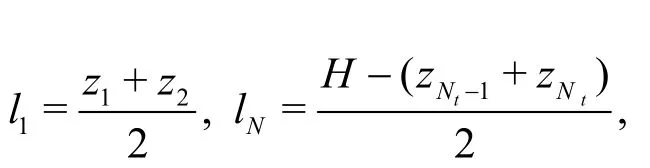
wherez1＜ z2＜ ···＜ zNt. For an ideal uniformity distri- bution, the value of UI should be zero (i.e., li=l, i = 1,2,···). However,it is not zero in practice because of the randomness of the molecular transport.

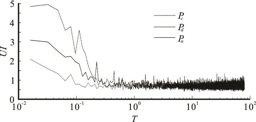
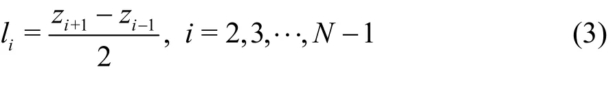
Fig.1 Development of transverse uniformity index ( )UI

As can be seen from Fig.1, the values of UI in three domains decrease and approach the asymptotic value of 0.7 at around =0.5T , i.e., the time to approach the transverse uniformity is =0.5T .

Besides, the longitudinal dispersion coefficient is time dependent in the early stage. Thus, some unreaso- nable explanations[7]were given to describe the results at the near-source region or in the early stage. Gill and Sankarasubramanian[8]shows that the longitudinal dispersion coefficient increases with time and reaches its asymptotic value at T =0.1-0.2. The numerical result of Gill and Sankarasubramanian[9]shows that the longitudinal dispersion coefficient in a pipe reaches its asymptotic value at =0.5T and that the timescale is independent of the initial transverse distribution.

In this letter, the longitudinal dispersion coeffi- cient is discussed in two aspects: the dimensionless history mean longitudinal transport coefficient ()K and the dimensionless temporal longitudinal transport coefficient (Kt). K is calculated as follows

whereastK is calculated as

The developments of K andtK (i.e., the curve (Ad andzD)) in Fig.2 show that the values of K andtK increase to their asymptotic values at =1.0T and =0.5T , respectively. The results by the Ad and Dzand Ad and Dxand Dzcombinations are similar. Therefore, the effect ofxD can be neglected when =100Pe . In Fig.2, the simulation curves including that obtained by the Ad andzD start to separate from the simulation curves including that obtained of the Ad when ＞ 0.10T . Therefore, the effect ofzD on K ortK becomes significant after T =0.1.

The longitudinal distribution is skew in the early stage. The result of Smith[10]shows that one sees a significant skewness when =1.0T .

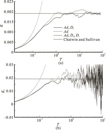
Fig.2 Simulations of K and tK, the theoretical solution of Chatwin and Sullivan[1] is also given

Fig.3 Developments of the skewness ()λ

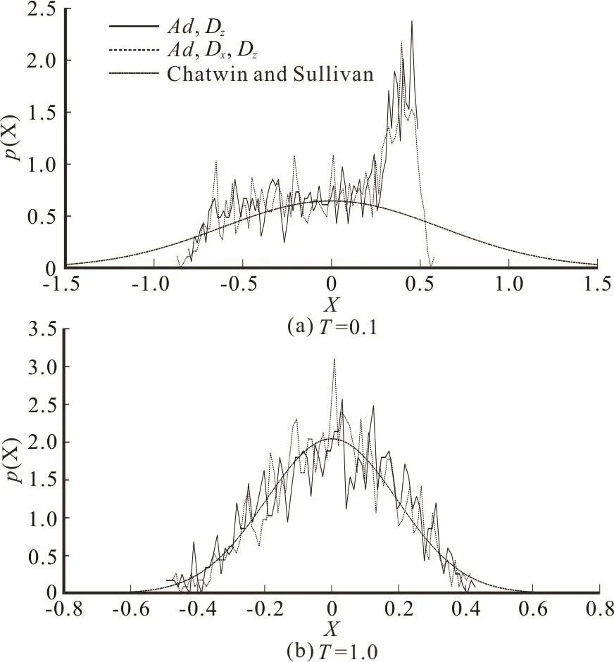
Fig.4 Illustrative diagrams of longitudinal distribution of the mean transverse concentration at =0.1T and =1.0T

As shown in Fig.3, the skewness is constant at 0.41 when only the advection is considered. The difference between curves obtained by the Ad and Dzand the Ad and Dxand Dzis marginal, the time λ approaches zero if T =1.0. From Fig.4, one can find that the difference between the numerical and theoretical results becomes obscure when =1.0T . In conclusion, a series of numerical simulations are conducted to give a comprehensive picture of the longitudinal scalar transport in the early stage. The early stage was usually treated as merely one stage when the Chatwin and Sullivan’s[1]solution cannot be used, without a detailed illustration of this stage. Here,we quantitatively study the process via the RWPM when Pe is large, and it is found that the early stage should be specifically divided into two detailed stages.The time transverse uniformity is approached if =T 0.5, and the time Gaussian longitudinal distribution is approached if =1.0T . These two timescales could help to form informed assumptions for the theoretical study of the scalar transport[11-15].

We are indebted to Dr. Daniel Fernandez-Garcia for his contributing suggestions and discussions. We are also indebted to Dr. Hansong Tang for commenting on the manuscript in a later stage.

[1] Chatwin P. C., Sullivan P. J. The effect of aspect ratio on longitudinal diffusivity in rectangular channels [J]. Journal of Fluid Mechanics, 1982, 120: 347-358.

[2] Noori R., Ghiasi B., Sheikhian H. et al. Estimation of the dispersion coefficient in natural rivers using a granular computing model [J]. Journal of Hydraulic Engineering,ASCE, 2017, 143(5): 04017001.

[3] Chatwin P. C. The initial dispersion of contaminant in Poiseuille flow and the smoothing of the snout [J]. Journal of Fluid Mechanics, 1976, 77: 593-602 .

[4] Bailey H. R., Gogarty W. B. Numerical and experimental results on the dispersion of a solute in a fluid in laminar flow through a tube [J]. Proceedings of the Royal Society of London A: Mathematical,Physical and Engineering Sciences, 1962, 269(1338): 352-367.

[5] Wu Z., Chen G. Q. Approach to transverse uniformity of concentration distribution of a solute in a solvent flowing along a straight pipe [J]. Journal of Fluid Mechanics, 2014,740: 196-213.

[6] Liang D., Wu X. A random walk simulation of scalar mixing in flows through submerged vegetations [J]. Journal of Hydrodynamics, 2014, 26(3): 343-350.

[7] Ananthakrishnan V., Gill W. N., Barduhn A. J. Laminar dispersion in capillaries: Part I. Mathematical analysis [J].AIChE Journal, 1965, 11(6): 1063-1072 .

[8] Gill W. N., Sankarasubramanian R. Exact analysis of unsteady convective diffusion [J]. Proceedingsof the Royal Society of London A: Mathematical, Physical and Engineering Sciences, 1970, 316(1526): 341-350.

[9] Gill W. N., Sankarasubramanian R. Dispersion of a nonuniform slug in time-dependent flow [J]. Proceedings of the Royal Society of London A: Mathematical, Physical and Engineering Sciences, 1971, 322(1548): 101-117.

[10] Smith R. Diffusion in shear flows made easy: The Taylor limit [J]. Journal of Fluid Mechanics, 1987, 175: 201-214.

[11] Li C. G., Xue W. Y., Huai W. X. Effect of vegetation on flow structure and dispersion in strongly curved channels[J]. Journal of Hydrodynamics, 2015, 27(2): 286-291.

[12] Wang Y. F., Huai W. X., Wang W. J. Physically sound formula for longitudinal dispersion coefficients of natural rivers [J]. Journal of Hydrology, 2017, 544: 511-523.

[13] Wang Y., Huai W. Estimating the longitudinal dispersion coefficient in straight natural rivers [J]. Journal of Hydraulic Engineering, ASCE, 2016, 142(11): 04016048.

[14] Gray F., Cen J., Shah S. M. et al. Simulating dispersion in porous media and the influence of segmentation on stagnancy in carbonates [J]. AdvancesinWater Resources,2016, 97: 1-10.

[15] Wu Z., Chen G. Q. Analytical solution for scalar transport in open channel flow: Slow-decaying transient effect [J].Journal of Hydrology, 2014, 519: 1974-1984.