Numerical analysis of cavitation shedding flow around a three-dimensional hydrofoil using an improved filter-based model＊

De-sheng Zhang (张德胜), Wei-dong Shi (施卫东), Guang-jian Zhang (张光建), Jian Chen (陈健), B. P. M. (Bart) van Esch

1.Research Center of Fluid Machinery Engineering and Technology, Jiangsu University, Zhenjiang 212013, China, E-mail:zds@ujs.edu.cn

2.Department of Mechanical Engineering, Eindhoven University of Technology, Eindhoven 5600MB, The Netherlands

Numerical analysis of cavitation shedding flow around a three-dimensional hydrofoil using an improved filter-based model＊

De-sheng Zhang (张德胜)1, Wei-dong Shi (施卫东)1, Guang-jian Zhang (张光建)1, Jian Chen (陈健)1, B. P. M. (Bart) van Esch2

1.Research Center of Fluid Machinery Engineering and Technology, Jiangsu University, Zhenjiang 212013, China, E-mail:zds@ujs.edu.cn

2.Department of Mechanical Engineering, Eindhoven University of Technology, Eindhoven 5600MB, The Netherlands

The cavitation shedding flow around a 3-D Clark-Y hydrofoil is simulated by using an improved filter-based model (FBM) and a mass transfer cavitation model with the consideration of the maximum density ratio effect between the liquid and the vapor. The unsteady cloud cavity shedding features around the Clark-Y hydrofoil are accurately captured based on an improved FBM model and a suitable maximum density ratio. Numerical results show that the predicted cavitation patterns and evolutions compare well with the experimental visualizations, and the prediction errors of the time-averaged lift coefficient, drag coefficient and Strouhal numberfor the cavitation number, the angle of attackat a Reynolds numberare only 3.29%, 2.36% and 9.58%, respectively. It is observed that the cavitation shedding flow patterns are closely associated with the vortex structures identified by thecriterion method. The predicted cloud cavitation shedding flow shows clearly three typical stages: (1) Initiation of the attached sheet cavity, the growth toward the trailing edge. (2) The formation and development of the re-entrant jet flow. (3) Large scale cloud cavity sheds downstream. Numerical results also indicate that the non-uniform adverse pressure gradient is the main driving force of the re-entrant jet, which results in the U-shaped cavity and the 3-D bubbly structure during the cloud cavity shedding.

Cloud cavitation, shedding flow, filter-based model, turbulent viscosity, Clark-Y hydrofoil

Introduction

Cavitation is a kind of complex phenomena involving phase transition, unsteadiness and multi-scale turbulence. It is well known that the strong instability of the cloud cavitation often leads to serious problems in hydraulic machinery, such as noise, vibration and erosion, etc.[1]. Most of these problems are related to the transient behavior of the cavitation structure, so the cavitation control is expected to improve the performance and the stability of the hydraulic machines[2,3]. With respect to the complex cavitating flows, many experiments were conducted to study the cloud cavitation, especially around the hydrofoils[4]and in venturitype sections[5]. The experimental results show that the initiation of the cloud cavitation begins with the formation of the re-entrant jet at the trailing edge of the attached cavity. The re-entrant jet inside the cavity is believed to be the cause of this cavity destabilization. When the re-entrant jet reaches the cavity leading edge, the cavity lifts off, breaks up, sheds and collapses downstream[6]. Although many interesting studies were reported with respect to these physical mechanisms, they are not yet fully understood because of the complex features of the unsteady cloud cavitation which interacts with the vortex structure in the wake.

Due to the complexity of the turbulent cavitatingflow, the numerical method becomes an important way to reveal related flow information, with the turbulence model for the cavitating flow remaining as an open issue. Many two equation turbulence models, such as the standardmodels, were employed to resolve the unsteady cavitation phenomena. However, it was shown that the Reynolds averaged Navier-Stokes (RANS) method cannot resolve the large scale turbulence structures, and its unsteady cavity prediction capability is also limited due to the over-prediction of the turbulent viscosity[2], which causes the re-entrant jet to lose momentum and makes it unable to cut across the cavity sheet. In order to solve the above over-prediction problem, the density corrected method (DCM) based on the local mixture density was proposed to limit the turbulent viscosity in the RNGturbulence model[7]. To improve the cavitation prediction accuracy, the large eddy simulation (LES), the direct numerical simulation (DNS), and the lattice Boltzmann method (LBM) were employed to model the unsteady cloud cavitation, which can offer some convincing time-dependent results. Ji et al.[8]and Luo et al.[9]used the LES model coupled with a mass transfer cavitation model to predict the unsteady threedimensional turbulent cavitating flow around a twist hydrofoil. However, the LES requires a very fine mesh, with a very heavy computational burden, and it is difficult to obtain a grid-independent solution[10]. Until now, the LES method has limited industrial applications, especially in hydraulic machines.

In recent years, hybrid models provide a solution for the over-prediction of the turbulent viscosity in the cavitating flow. Taking into account the advantages of the RANS and the LES, Johansen et al.[11]proposed a filter-based model (FBM) blending the RANS and LES models to calculate the wake flow of the square object, and obtained results with a higher prediction accuracy. Many validations[11,12]were made for the hybrid FBM for the cavitating flows in a square cylinder, a hydrofoil and a hollow-jet valve. The results show the FMB can better capture the unsteady features of the cavitating flows than the normal RANS models. However, the FMB is not effective in the near-wall region. It indicates that the two equation model will be over-covered when the filter size. Furthermore, the filter scale in the FBM and the maximum density ratio in the cavitation model have important effects on the numerical results[11-13].

In view of the success of their studies, this paper analyzes the cavitation shedding flow around a 3-D Clark-Y hydrofoil using an economical and accurate simulation method, which employs the modified FBM turbulence model and the homogeneous cavitation model. Especially, the filter scale, the maximum density ratio, and the DCM are considered to improve the prediction accuracy. The unsteady features of the cavitation shedding flow are analyzed by both numerical and experimental results.

1. Numerical method and setup

1.1Governing equations

In the vapor/liquid two-phase mixture model, the fluid is assumed to be homogeneous, so the multiphase fluid components are assumed to share the same velocity and pressure. The continuity and momentum equations for the mixture flow are:

1.2Filter-based density correction method

The original two-equation models may over-predict the turbulent viscosity in the cavitation region, causing the re-entrant jet to lose momentum and making it unable to cut off the attached cavity. To improve the simulations by taking into account the influence of the local compressibility effect on the turbulent closure model, the DCM based on the local mixture density was proposed by Reboud et al.[5], and then Coutier-Delgosha et al.[4]indicated that the DCM could help to reduce the turbulent viscosity in the RNGturbulence model.

Fig.1 (Color online) Predicted time-averagedaround a Clark-Y hydrofoil at

The filter-based model (FBM)[11]is based on the original RNGturbulence model. In this paper, a filter-based density corrected model is proposed, which combines the strengths of both the FBM and DCM models. A hybrid method for the filter functionand the DCM is added in the kinematic eddy viscosity equation to reduce the turbulent viscosity and limit the over-prediction in the cavitating flow on the hydrofoil wall and in the wake[5].

1.3Cavitation model

The cavitation model describes the mass transfer between the liquid and the vapor. The present paper employs the Zwart-Gerber-Belamri cavitation model derived from a simplified Rayleigh-Plesset equation which neglects the second-order derivative of the bubble radius. The vapor density is clipped in a usercontrolled fashion by the maximum density ratioto control the numerical stability and the accuracy[14]. The maximum density ratio is used to clip the vapor density for all terms except the cavitation source term itself, which is determined by the true density specified as the material property.

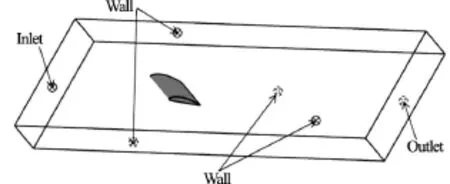
Fig.2 Computational domain and boundary conditions

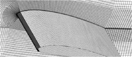
Fig.3 The structural mesh around the Clark-Y hydrofoil

The vapor volume fraction is governed by the following equations:

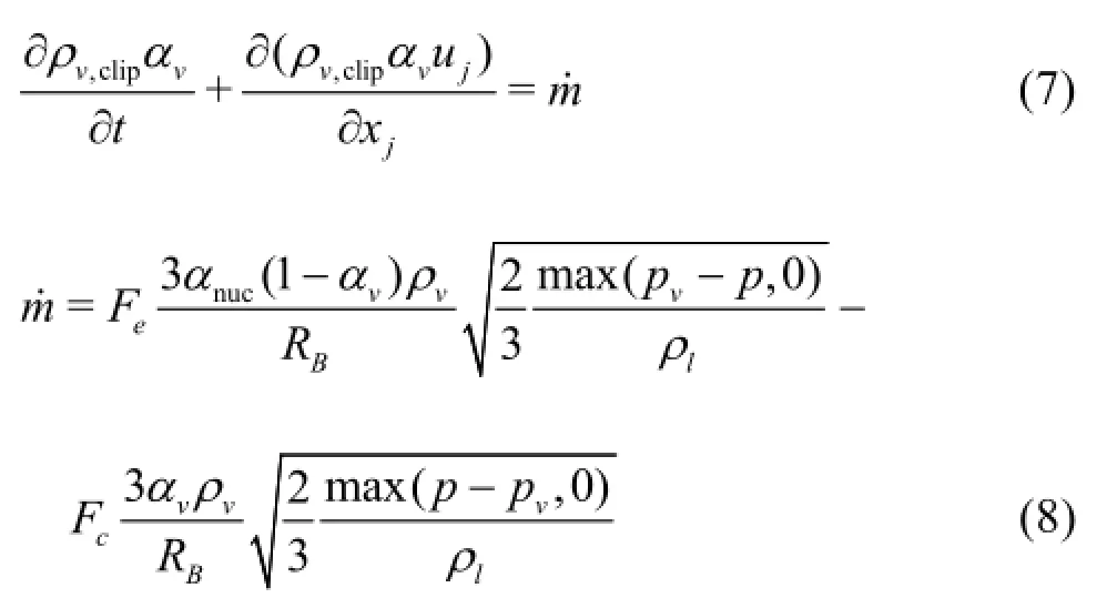
Table 1 Results of the mesh independence study,, non-cavitation

Table 1 Results of the mesh independence study,, non-cavitation

1.4Numerical setup and description

The computational domain and the boundary conditions are decided according to the experimental setup[8], as shown in Fig.2. The Clark-Y hydrofoil is fixed in the center of the water channel at the angle of attack. A no-slip wall is imposed on the hydrofoil surface, and the wall conditions are imposed on the top and bottom boundaries of the tunnel. The inlet velocity is set to becorresponding to the Reynolds numberThe outlet pressure is determined by the cavitation number. The total grid elements are 17 748 150 as shown in Fig.3, and the range ofvalue is from 1 to 32.

The simulations are conducted by using the CFD code ANSYS CFX. The pressure-velocity direct coupling method is used to solve the governing equations. The high resolution scheme is used for the convection terms with the central difference scheme used for the diffusion terms in the governing equations. The unsteady second-order implicit time integration scheme is used for the transient term. The unsteady cavitating flow simulations are started from a steady non-cavitation flow results. The time stepfor the revolution calculation. During the unsteady calculation, the convergence in each physical time step is achieved with 4 to 10 iterations when the root mean square (rms) residual is dropped to a value below 10−5.

The influence of the grid node number on the simulation results is validated using three kinds of grids with different mesh numbers. The results of the mesh independence study are presented in Table 1. The results predicted by the mesh cases of Refined 1 and Refined 2 all compare well with the experiment results. A good agreement of the pressure coefficientdistribution between the experimental data and the predicted results using the improved numerical method and the mesh case of Refined 2 is shown in Fig.4 and Table 1, so the mesh of Refined 2 is used in the present simulations.

Fig.4 Pressure coefficient distribution on Clark-Y hydrofoil,, non-cavitation

Fig.5 Time-averaged velocity

Table 2 Comparison of the time-averaged measured and predicted lift coefficientsand drag coefficientsfor

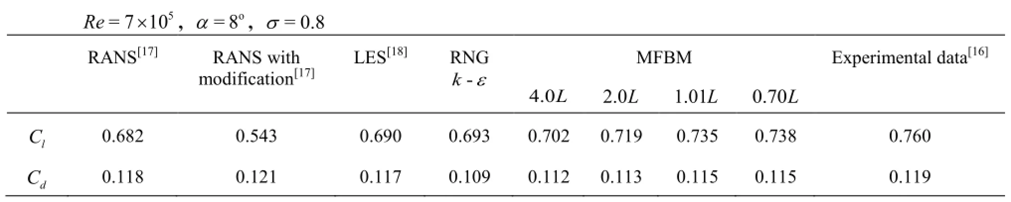
Table 2 Comparison of the time-averaged measured and predicted lift coefficientsand drag coefficientsfor

?

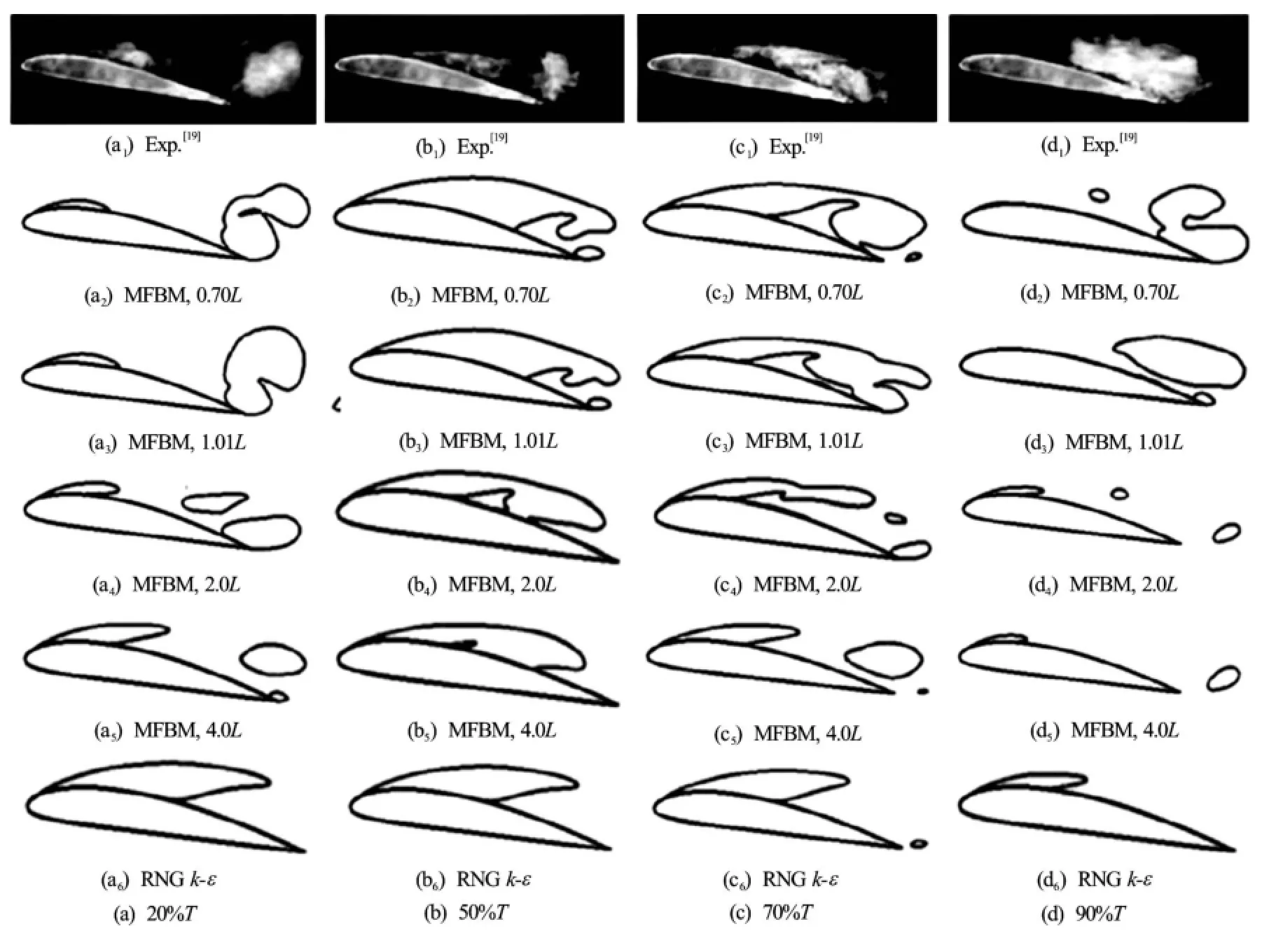
Fig.6 Comparison of experimental and numerical cavity patterns predicted by different turbulence models and filter sizes, cavity patterns are visualized by iso-contour of

2. Results and discussions

2.1Effect of the filter scale

As shown in Fig.5, the horizontal coordinate is the velocityuatwhich is monitored to see the influences of the different filter scales.

Table 3 Comparison of the effect of the maximum density ratio,

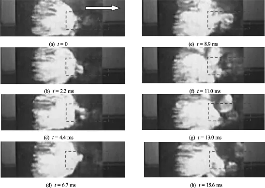
Fig.7 Experimental sheet cavity patterns (). The arrow indicates main flow direction

Fig.8 (Color online) Predicted cavity patterns and local velocity vector distributions with different

The cloud cavity shedding results in a wake flow near the trailing edge (TE), where the flow velocity is in a parabolic distribution. As shown in Fig.5, the numerical results obtained by the RNGmodel has a large prediction error as compared with the experimental data. With the decrease of the filter size, the difference gradually decreases. When the filter size decreases to, the results are almost stable. It indicates that the RNGmodel cannot capture the shedding flow with the large-scale vortex, but the FBM model can and effectively.

Table 2 shows the predicted time-averaged lift and drag coefficients of five cycles calculated by using different filter scales and other numerical results[17,18]. With the decrease of the filter scale, the time-averaged lift and drag coefficients gradually approachthe experimental data based on the DCM and a maximum density ratio of 20 000. From the comparison in Table 2, one sees a better agreement of the numerical data in the present study with the experimental results than the RANS results. The numerical results simulated by using the FBM with a filtercan achieve the accuracy level of the LES prediction results[18].

To better understand the effect of the filter scale on the unsteady cavity patterns, Fig.6 illustrates a comparison of the predicted cavity patterns atby using the originalmodel and the MFBM with different filter scales. As seen in the experimental images, the unsteady cavity shedding flow occurs in one cycle at, while no cavity shedding process shows in the results simulated by the original RNGmodel.The more obvious shedding phenomenon of cavitation occurs when, but the cavity length and thickness are smaller as compared with the experimental results, and the vapor-liquid interface is relatively uniform and steady. With the decrease of the filter scale, the cavitation characteristics become unsteady and unstable. When, the large-scale cavity shedding phenomenon appears, and the cavity patterns and evolutions are consistent with the experimental images. It indicates that the MFBM model can simulate the cloud cavitation features more accurately than the original RANS models. However, ifis further reduced, the evolution of the cavity changes very little, mainly due to the limitations of the grid size. It should be pointed out that the further reduction of the filter scale will resolve the small scale turbulence structures, but the current grid resolution is unable to meet the requirements to reach the LES level. In general, an appropriate filter scale in the FBM is critical for the prediction accuracy. The smaller filter size could increase the correction capability of the FBM model. On the whole, the capability of the FBM model is limited by the grid size and the computation resource. The filter sizeis used in the present simulations.

2.2Effect of maximum density ratio

In order to ensure that the simulation is stable, the maximum density ratiois introduced to control the vapor density.is substituted into Eq.(7), we obtain

Equation (7) shows that the cavitation mass transfer rate (the righthand side term) has a close relation with the maximum density ratio. It was suggested in previous studies[19]thatcan affect the compressibility in the vapor-liquid mixture region and the vapor-liquid transfer rate. With the increase of the maximum density ratio, the length of the cavity calculated by using the default value of 1 000 in ANSYS CFX is almostas shown in Table 3, so we have a large perdition error as compared with the experiment value of. The lift coefficient, the drag coefficient, the cavity area and the cavity length all increase with the increase of the maximum density ratio. When the maximum density ratio reaches 20 000 or 43 197, the numerical difference is quite small, and the predicted results are all close to the experimental results[16]. Morgut et al.[19]also indicated that the default value of the cavitation model in the ANSYS CFX codes under-predicts the development of the cavity.

Figure 7 presents the experimental visualizations[4]on the Clark-Y hydrofoil with the cavitation numberThe sheet cavity is attached on the suction side of the hydrofoil from the leading edge to the place ofThe body of the cavity is stable, but the rear region of the sheet is unsteady, 3-D, and it rolls up into a series of bubbly eddies that shed intermittently. The steady attached sheet cavity in Fig.8 is obtained with the default maximum density ratio of 1 000, but the circulation flow in the region A is not observed. The larger value ofpromotes the mass transfer rate between the liquid phase and the vapor phase, which results in a significant rise of the vapor fraction inside the cavity as shown in Fig.8. From the numerical results predicted by the maximum density ratios of 20 000 and 43 197, the quasi-unsteady sheet cavity is also observed, with the clockwise vortex induced by the interaction of the re-entrant jet and the main flow at the closure of the cavity as shown in the region A. Disturbed by the vortex, the small bubble clusters are shed from the rear part of the cavity, as is consistent with the experiment results in Fig.6.

Fig.9 (Color online) Contour distributions of mass transfer source term predicted by different maximum density ratios,

In order to further see the effect of the maximum density ratio on the mass transfer rateFig.9 illustrates the contour distributions of the mass transfer source term simulated by the max density ratiosrespectively. Theevaporation of the liquid phase to the vapor phase is positive, and the condensation is negative. The evaporation process mainly occurs on the leading edge sheet cavity of the hydrofoil, while the condensation process primarily occurs in the rear of the sheet cavity. With the increase of the maximum density ratio, the process of the phase transition is promoted and the mass transfer rate between the liquid and the vapor phase sees a significant increase in the cavity, and the cavity length and thickness are also increased as shown in Figs.9(b) and 9(c). Thus, the mass transfer from the liquid to the vapor at a higher maximum density ratio can produce a larger vapor cavity volume under the same operating conditions. They can be noted in the cavitation simulation.

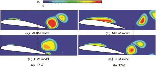
Fig.10 (Color online) Comparison of cavity shapes predicted by using different turbulence models,

Fig.11 (Color online) Distributions of turbulent viscosity calculated by different turbulence models,

In the present study, it is found that the default valuecould ensure the numerical stability and accelerate the convergence of the calculation, but the development of the cavitation is underestimated. As a balance between the prediction accuracy and the convergence, the suitable maximum density ratio of 20 000 is employed in this paper.

2.3Effect of density correction method on cavity pattern

In order to compare the MFBM model with the original FBM model, an unsteady simulation is carried out for the cloud cavitation around the hydrofoil using the two different turbulence models, and the simulation results are shown in Fig.10. The two turbulence models could reproduce the cloud cavity shedding due to the FBM employed in the simulation of the hydrofoil. The main difference between the two predicted results is the sheet cavity length and the vapor volume fraction inside the cavity. The original FBM model is based on themodel, which normally overpredicts the turbulence viscosity inside the mixture of the vapor and the liquid, because the higher energy dis-sipation severely limits the growth of the cavity near the leading edge when, i.e., when the local mesh size is much greater than the turbulence length scale. However, the MFBM model takes into account the turbulent viscosity correction of the mixture based on the DCM, which could generate a reasonable bubble growth and the cavity length and the vapor volume fraction inside the cavity could be increased as well.

Figure 11 shows the turbulent viscosity distribution obtained by using different turbulence models. The originalmodel over-predicts the turbulent viscosity in the cavity regions, which would hinder the sheet cavity fracture and the cloud cavity shedding. As mentioned in Section 2.2, the FBM model can reduce the over-estimation of the turbulent viscosity, especially in the regions with large turbulence scales. From Eq.(6) of the FBM, the flow field with a large turbulence scale is simulated by using the LES single-equation, which predicts a more reasonable turbulent viscosity. However, the FBM model still has some limitations, e.g., in the small-scale turbulent region and the near wall region, themodel is recovered. It means that the traditional two-equation turbulence model is used for the simulation without taking into account the compressible effects of the vapor-liquid region. To solve this problem, the DCM is applied in the FBM. With the FBM combined with the DCM, a reasonable distribution of the turbulent viscosity could be predicted, as shown in Fig.11(c). The predicted unsteady features of the cloud cavitation also agree well with the experimental visualizations in the following simulations.

The pressure distribution on the surface of the hydrofoil is closely related with the cavity growth, shedding and collapse, so the lift and drag coefficients should have a quasi-periodic behavior against the change of the cavity pattern. To validate the predicted results obtained by using the MFBM model, the lift coefficientand the drag coefficientare monitored in an unsteady simulation. Figure 12 presents the comparison of the time evolutions of the experimental and numerical lift coefficientand the drag coefficientin three cycles. As shown in Fig.12, there are some differences between the numerical lift coefficient curve and the experimental data, which is because the high frequency fluctuation in the bubble breakdown is failed to be captured in the experimental measurement. The numerical time-averaged lift and drag coefficients are 0.735 and 0.119, respectively, and the prediction errors are only 3.29% and 3.36%, as compared with the experimental valuesand. The results are more accurate than the RANS results[17].

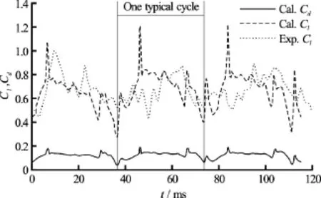
Fig.12 Time evolutions of lift and drag coefficients in the cavitation shedding flow, MFBM,

Fig.13 Frequency spectrum of lift coefficient in cloud cavitation calculated by numerical simulation

The predicted time-dependent lift coefficient is processed by using the Fast Fourier Transformation, and the spectrum analysis of the lift coefficient is shown in Fig.13. The main frequency is normalized by the chord lengthand the upstream velocity. The predicted primary oscillating frequencycompares well with the experimental valueThe primary frequency of the hydrodynamic fluctuations is induced by the unsteadiness of the cavity, as in agreement with thecloud cavity shedding frequency, which is validated in the present simulations. The predicted second oscillating frequencyis also quite near the experimental value. The second frequency may be due the instability of the vortex structures interacted with the unsteady cavitation shedding flow.

Fig.14 Comparison of cavity pattern evolutions in one cycle

It is well known the sheet and cloud cavitations are highly turbulent and unsteady, especially when the cloud cavity shedding flow happens. In order to better see how the improved method has captured the unsteady dynamics, Fig.14 shows the comparison of the predicted time-dependent evolutions of the cavity patterns and the experimental visualizations at0.8. It is observed that the predicted cloud cavitation has a distinct quasi-periodic pattern, and the cavity visualizations are in side views according to 5%, 11%, 20%, 63%, 70%, 81%, 90% and 97% of each corresponding cycle. The cycle lengthTof the cloud cavitation is estimated as 38.3ms, which is near the experimental result ofThe predicted patterns of every stage during the unsteady cloud cavitation generally agree well with the experimental visualizations including the initiation of the attached cavity, the growth toward the trailing edge, and the subsequent cloud shedding[21], and some tiny discrepancies are because of the inherent assumption of the cavitation model such as the compressibility and the bubble cloud effects. As shown in Fig.14, first of all, the attached sheet cavity expands up to the TE of the hydrofoil atfollowed by the breakup near the LE due to the re-entrant jet atand then the complete convection of the cloud cavity into the wake at

Fig.15 (Color online) Comparison of cavity patterns obtained by experiment and simulation, MFBM,

2.43-D cavitation shedding flow around Clark-Y hydrofoil

Figure15(a) shows the experimental visualizations of the 3-D cavitation shedding flow, which has a very distinct quasi-periodic feature. In order to illustrate the evolution of the 3-D shedding vortex structure effectively, the side view of the cavity shedding is shown by plotting of the vapor volume fraction iso-surfaces ofin one cycle as shown inFig.15(b). The vortex structures in the cavitation shedding flow are visualized based on thecriterion to identify the vortices. Positive values of thecriterion, defined as the second invariant of the velocity gradient tensor, are given by

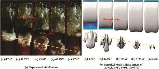
Fig.16 (Color online) Collapse process of cloud cavity

Figure 15 illustrates the correlation between the vortex structure and the cloud cavity in one cycle. For predicting the three-dimensional vortex structure in the present case, the iso-surface of thecriterion with the value of 150 000 s-2is used to visualize the turbulent cavitating flow. From Figs.15(a)-15(c), we can clearly observe the cavity shedding process and more scales of the vortices as well as the formation of the U-shaped cavity. The features of every stage of the experimental visualizations are well captured. Based on both experimental and numerical results of the cavity and thecriterion, the unsteady cloud cavitation in one cycle could be divided into the following stages: (1) Initiation of the attached cavity, the growth toward the trailing edge. The first stage is the growth of the attached cavity immediately from 0 to 45% after a cloud cavity shedding. The numerical results presented in Figs.10(b) and 10(c) show a close correlation between the cloud cavity and the vortices structures, which indicates that the vortices structure is an important mechanism for the cavity shedding flow generation. The complicated vortex structures with a large eddy scale makes the shedding flow seem much more unsteady as compared with the iso-surface of the cavity, as in agreement with the experiment. (2) The formation and development of the re-entrant flow. Figure 15presents the evolution of the cavity patterns and the development of the re-entrant jet in the second stage of one cycle. Atthe attached sheet cavity grows to its maximum length, and the cavity interface becomes bubbly. The adverse pressure gradient is strong enough to overcome the weaker momentum of the flow confined by the nearwall region, so a re-entrant jet forms and begins to move upstream at this time point. Atthe U-shaped cavity occurs on the surface of the hydrofoil owing to the effects of the side-wall. (3) Large scale cloud cavity sheds downstream. Atand, the re-entrant flow reaches the vicinity of the cavity leading edge, and the sheet cavity is lifted away from the hydrofoil surface and sheds downstream in the form of the cloud cavity. The complex vortex structures visualized by thecriterion are extremely unsteady and unstable near the TE due to the unsteady partial breakup and collapse. The oscillating trailing edge vortex pair (A) is observed at the same time, and the cloud cavity is convected into the wake and collapses.

The comparison of the predicted and experimental evolutions of the cloud cavity shedding and collapse process[22]is shown in Fig.16. It is similar to the typical cloud cavity transformation observed in Ref.[23]. The cloud cavity is detached from the hydrofoil surface, and then it is entrained downwards by the main flow, finally collapses in the wake. The shedding speed of the cloud cavity predicted by the center position of the cloud cavity and the time interval in the experiment images is approximatelyThe predicted instant cavity collapse process compares well with the experimental observations, but the numerical shedding speed of the cloud cavity is near. Maybe the prediction error is caused by the compressibility and the bubble cloud effects not included in the present simulation. Reference [24] indicated that the shedding vapor is in the form of bubble clusters, which will influence the fluid compressibility and the wave speed, and affect the collapsing behavior. It is noted that the primary cloud cavity has a large bubbly structure owing to the non-uniform re-entrant jet, which is responsible for the breakup, the subsequent shedding and collapse of the separated cloud cavity. Experimental and simulation results all indicate that the cloud cavity is distorted into a U-shaped cavity structure under the 3-D effects of the side-wall as it moves downward, and then splits into the two symmetrical cavities, which finally collapse in the wake.

Figure 17 illustrates the pressure contours and the U-shaped cavity pattern visualized by the iso-surface ofin the top view of the hydrofoil atThe adverse pressure gradient is responsible for the re-entrant jet, and it plays a key role in the dynamics of the cavitation. Atthe re-entrant jet moves backwards and encounters the main flow at a place of about 30% chord where the local pressure is high. The local high pressure looks as in a U-shaped distribution, due to the effect of the side-wall. In order to better see the pressure distribution on the 3-D Clark-Y hydrofoil, Fig.18 shows the detailed pressure distribution at three cross-sections. The peak of the local high pressure corresponding to the U-shaped pressure occurs atand the adverse pressure gradient at the middle span is much larger than that atwhich will determine the front location of the re-entrant jet. It should be pointed out that the local high pressure will contribute to the vapor condensation as illustrated in Fig.9, and results in the cutoff of the attached cavity. It also indicates that the side-wall of the hydrofoil is also an important factor which affects the cloud cavity shedding.

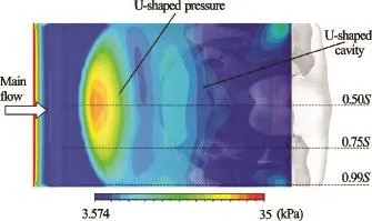
Fig.17 (Color online) Top view of cavity shape visualized by the iso-surface of vapor volume fractionand pressure contours at

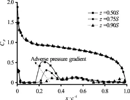
Fig.18 Pressure coefficient distributions along the surface of Clark-Y hydrofoil at

In order to find the correlation between the U-shaped cavity and the re-entrant jet, Fig.19 presents the in-plane velocity vector distributions at different spans. The locations of the front of the re-entrant jet at the same instant time at the spansare different because of the different adverse pressure gradient. The front location of the re-entrant jet atis at a place of about 20% chord of the hydrofoil, and and that atis at a place of about 30% chord, while that atis at a place of near 40% chord. The U-shaped pressure distribution as shown in Fig.14 results in the non-uniform re-entrant jet in the span direction. Thus, the strength difference of the re-entrant jet is the main reason for the formation of the U-shaped cavity.

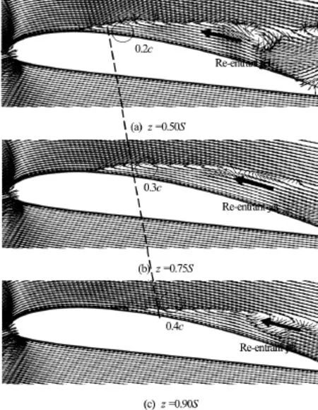
Fig.19 Re-entrant jets at different spans at

3. Conclusions

The work of this paper is based on the 3-D Clark-Y hydrofoil by using an improved FBM turbulence model and the homogeneous cavitation model with the optimal maximum density ratio. The numerical results compare well with the experiment data, and the following conclusions can be drawn:

(1) The influences of the filter scale, the maximum density ratio and the density correction method on the unsteady cloud cavitation shedding flow are studied in detail. The maximum density rate could affect the mass transfer rates between the liquid and the vapor. The turbulent viscosity correction based on the filter-based density correction method could improve the cavity length and the vapor fraction inside the cavity. Numerical results have well captured the unsteady features of the cloud cavitation in one cycle based on the improved numerical method. The prediction errors of the time-averaged lift coefficient, the drag coefficient and the Strouhal number are only 3.29%, 2.36% and 9.58%, respectively as compared with the experimental data.

(3) The collapse process and the U-shaped cavity are well-captured in the cavitation shedding flow around the 3-D Clark-Y hydrofoil, which compares well with the experimental visualizations. It is found that the adverse pressure gradient, as the main driving force of the generation of the re-entrant jet, varies with the different spans owing to the viscous resistance of the side-wall. The non-uniform re-entrant jet in the span direction is the main cause of the formation of the U-shaped cavity, which also results in the 3-D large scale bubbly structure of the cavity cloud during the shedding process.

[1] Luo X. W., Ji B., Tsujimoto Y. A review of cavitation in

[2] Leroux J. B., Coutierdelgosha O., AstolfiJ. A. A joint hydraulic machinery [J].Journal of Hydrodynamics, 2016, 28(3): 335-358. experimental and numerical study of mechanisms associated to instability of partial cavitation on two-dimensional hydrofoil [J].Physics of Fluids, 2005, 17(5): 052101.

[3] Zhang D., Shi L., Shi W. et al. Numerical analysis of unsteady tip leakage vortex cavitation cloud and unstable suction-side-perpendicular cavitating vortices in an axial flow pump [J].International Journal of Multiphase Flow,

[4] Coutier-Delgosha O., Reboud J. L., Delannoy Y. Numeri-2015, 77: 244-259. cal simulation of the unsteady behaviour of cavitating flows [J].International Journal for Numerical Methods in Fluids, 2003, 42(5): 527-548.

[5] Reboud J. L., Stutz B., Coutier-Delgosha O. Two phase flow structure of cavitation: Experiment and modeling of unsteady effects [C].Proceedings of the Third Symposium on Cavitation. Grenoble, France, 1998.

[6] Johansen S. T., Wu J., Wei S. Filter-based unsteady RANS computations [J].International Journal of Heat and Fluid Flow, 2004, 25(1):10-21.

[7] Kim S., Brewton S. A multiphase approach to turbulent cavitating flows [C].Proceedings of 27th Symposium on Naval Hydrodynamics. Seoul, Korea, 2008.

[8] Ji B., Luo X. W., Peng X. X. et al. Three-dimensional large eddy simulation and vorticity analysis of unsteady cavitating flow around a twisted hydrofoil [J].Journal of

[9] Luo X. W., Ji B., Peng X. X. et al. Numerical simulationHydrodynamics, 2013, 25(4): 510-519. of cavity shedding from a three-dimensional twisted hydrofoil and induced pressure fluctuation by large-eddy simulation [J].Journal of Fluids Engineering, 2012, 134(4):

[10] Moin P. Advances in large eddy simulation methodology 041202. for complex flows [J].International Journal of Heat and Fluid Flow, 2002, 23(5):710-720.

[11] Johansen S. T., Wu J., Wei S. Filter-based unsteady RANS computations [J].International Journal of Heat and Fluid Flow, 2004, 25(1): 10-21.

[12] Huang B., Wang G. Y. Evaluation of a filter-based model for computations of cavitating flows [J].Chinese Physics Letters, 2011, 28(2): 026401.

[13] Zhang D. S., Wang H. Y., Shi W. D. et al. Numerical analysis of the unsteady behavior of cloud cavitation around a hydrofoil based on an improved filter-based model [J].Journal of Hydrodynamics,2015, 27(5): 795-808.

[14] Ji B., Luo X., Wu Y. et al. Partially-averaged Navier-Stokes method with modified -kε, model for cavitating flow around a marine propeller in a non-uniform wake [J].International Journal of Heat and Mass Transfer, 2012, 55(23-24): 6582-6588.

[15] Mejri I., Bakir F., Rey R. et al. Comparison of computational results obtained from a homogeneous cavitation model with experimental investigations of three inducers [J].Journal of Fluids Engineering, 2006, 128(6): 1308-1323.

[16] Wang G., Senocak I., Wei S. et al. Dynamics of attached turbulent cavitating flows [J].Progress in Aerospace Sciences, 2001, 37(6): 551-581.

[17] Wei Y. J., Tseng C. C., Wang G. Y. Turbulence and cavitation models for time-dependent turbulent cavitating

[18] Huang B., Zhao Y., Wang G. Large eddy simulation of flows [J].Acta Mechanica Sinica, 2011, 27(4): 473-487. turbulent vortex-cavitation interactions in transient sheet/ cloud cavitating flows [J].Computers and Fluids, 2014, 92(3): 113-124.

[19] Morgut M., Nobile E., Bilus I. Comparison of mass transfer models for the numerical prediction of sheet cavitation around a hydrofoil [J].International Journal of Multiphase Flow, 2011, 37(6): 620-626.

[20] Ji B., Luo X., Wu Y. et al. Numerical analysis of unsteady cavitating turbulent flow and shedding horse-shoe vortex structure around a twisted hydrofoil [J].International Journal of Multiphase Flow, 2013, 51(5): 33-43.

[21] Huang B. Physical and numerical investigation of unsteady cavitating flows [D]. Doctoral Thesis, Beijing, China: Beijing Institute of Technology, 2012(in Chinese).

[22] Huang B. Wang G. Y., Zhao Y. et al. Physical and numerical investigation on transient cavitation flows [J].Science China Technological Sciences,2013, 56(9): 2207-2218.

[23] Kawanami Y., Kato H., Yamaguchi H. et al. Mechanism and control of cloud cavitation [J].Journal of Fluids Engineering, 1997, 119(4): 788-794.

[24] Foeth E. J., Terwisga T. V., Doorne C. V. On the collapse structure of an attached cavity on a three-dimensional hydrofoil [J].Journal of Fluids Engineering, 2008, 130(7): 933-943.

(Received June 4, 2016, Revised December 16, 2016)

* Project supported by the National Natural Science Foundation of China (Grant No. 51479083), the Prospective Joint Research Project of Jiangsu Province (Grant No. BY2015064-08), The Primary Research and Development Plan of Jiangsu Province (Grant Nos. BE2015001-3, BE2015146) and the 333 Project of Jiangsu Province and Six Talent Peaks

Project in Jiangsu Province (Grant No. HYGC-008).

Biography: De-sheng Zhang (1982-), Male, Ph. D., Professor