
Feature-aligned segmentation using correlation clustering
2017-06-19 19:20YixinZhuangHangDouNathanCarrandTaoJu
Computational Visual Media 2017年2期
Yixin ZhuangHang Dou,Nathan Carr,and Tao Ju
Feature-aligned segmentation using correlation clustering
Yixin Zhuang1Hang Dou2,Nathan Carr3,and Tao Ju2
We present an algorithm for segmenting a mesh into patches whose boundaries are aligned with prominent ridge and valley lines of the shape.Our key insight is that this problem can be formulated ascorrelation clustering(CC),a graph partitioning problem originating from the data mining community. The formulation lends two unique advantages to our method over existing segmentation methods.First, since CC is non-parametric,our method has few parameters to tune.Second,as CC is governed by edge weights in the graph,our method offers users direct and local control over the segmentation result.Our technical contributions include the construction of the weighted graph on which CC is defined,a strategy for rapidly computing CC on this graph,and an interactive tool for editing the segmentation.Our experiments show that our method produces qualitatively better segmentations than existing methods on a wide range of inputs.
mesh segmentation;correlation clustering (CC);feature lines
1 Introduction
Surface segmentation is one of the fundamental problems in geometry processing.A semantically meaningfulsegmentation has important applications in parameterization,texturing,and shape matching.For many real-world objects,particularly man-made shapes,their semantics are well captured by linetype features,particularly ridges and valleys[1].As a result,it is naturalto require that the segmentation of such objects shouldalign with their feature lines.Feature-aligned segmentation has enabled applications such as shape abstraction[2,3]and interactive wire-based deformation[4].
Despite extensive research into segmentation,few works have specifically addressed feature-aligned segmentation.Patch-based segmentation methods are mostly concerned with finding patches that meet certain regularity criteria,such as being well-fit by primitives or having homogeneous curvature.While the resulting patch boundaries often coincide with feature lines,it is common for these methods to ignore prominent feature lines or create redundant patches within featureless regions(Figs.1(b)and 1(c).Only a few methods explicitly aim to preserve a given set of feature lines as the patch boundaries[7, 8].However,they all rely on heuristics that involve multiple parameters.We have found that in practice it is often difficult,ifnot impossible,to find the right parameter values to keep salient features without adding redundant boundaries in featureless regions (Fig.1(d)).
We propose a new method for feature-aligned segmentation.We explicitly formulate as the goal toinclude as many prominent feature lines and as few weak feature or non-feature lines as possible, as patch boundaries.This is a classical graph partitioning problem known ascorrelation clustering(CC)[9].A distinctive property of CC is that it is able to automatically recover the number of clusters.This is achieved by associating graph edges withsignedweights.We show how feature-aligned mesh segmentation can be cast as a CC problem by defining an appropriate weighted graph on themesh.In addition,we show how state-of-the-art solvers for CC can be significantly sped up in our problem setting,with little loss of accuracy,by precomputing an oversegmentation of the mesh guided by our graph weights.

Fig.1 Comparisons of patch-based segmentation of(a)the Rockerarm created by(b)the primitive-fitting method of Yan et al.[5], (c)the region-growing method of Nieser et al.[6],(d)the curvaturesimilarity guided method of Mitani and Suzuki[7]obtained from the ridge(red)and valley(blue)lines in(a),and(e)our method(withα= 0.6),using the same set of feature lines.Note that existing methods often miss prominent features(see blue boxes)or produce too many segments in featureless regions(see red boxes).Our method captures the majority of the prominent features without creating redundant segments.
We have observed in extensive experiments that our segmentation method outperforms existing methods in maximizing inclusion of prominent feature lines while avoiding redundant patches in featureless regions(Fig.1(e)).Moreover,the CC formulation and our efficient solver enable intuitive editing interfaces where the user can locally refine or coarsen the segmentation with instant feedback.
Although CC has been used for related problems including image segmentation and part-based mesh segmentation[10],it has not been used for featurealigned mesh segmentation.We make the following three technical contributions:
•We formulate feature-aligned segmentation in terms of CC.In particular,we design graph weights such that the cluster boundaries of CC are made up of salient feature lines connected by shape-following paths(see Section 3.2).
•We give an efficient CC algorithm based on precomputing an oversegmentation from the feature lines.We show that our oversegmentation,which is tailored to our graph,yields quantitatively better results than existing oversegmentations(see Section 3.3).
•We provide an interactive interface for modifying the segmentation that benefits from our CC formulation and the efficiency of our algorithm (Section 4).
2 Related work
2.1 Surface segmentation
We briefly cover the extensive research on this topic, with an emphasis on its ability to produce featurealigned segmentations.We refer readers to excellent surveys[11,12]for more in-depth discussions ofthese and other works.
Segmentation methods generally fall into two camps,being eitherpart-basedorpatch-based.The first camp aims to partition a solid object into volumetric components.They utilize part-aware shape descriptors such as concavity of the cuts[13, 14],convexity[15,16]of parts,compactness[17] of parts,a shape diameter function[18],or a combination of these[19,20].More sophisticated descriptors can be learned from a collection of shapes[21].
The second camp of methods,to which our method belongs,offers a more detailed partitioning of the surface.For our purpose,we classify patchbased segmentation methods intoimplicitandexplicitschemes.Implicit schemes seek patches that satisfy certain regularity conditions.Ideally,the feature lines emerge implicitly as the boundaries of the patches.The regularity condition can be low approximation error by an analytical primitive[5, 22–25],developability[26,27],or similarity using a variety of shape descriptors,including curvature[6, 28–31],normal voting tensor[32],slippage[33],and diffusion-type distances to a set ofseed locations[34, 35].However,implicit methods can oversegment surface regions that are void of prominent feature lines,if the region fails the regularity conditions.For example,the region could assume a shape more general than the space of allowed primitives or exhibit significant variation of curvature due to noise(as in the red boxes in Figs.1(b)and 1(c)). Moreover,a prominent feature line can be missed in the segmentation,if the feature line is surrounded by a region of surface with homogenuous appearance (as in the blue boxes in Figs.1(b)and 1(c)).
Explicit schemes start from a given set of feature lines and seek to create patches that are bounded by strong features.Existing explicit methods[7,8,36]start by pruning away weak feature lines.Afterwards,L´evy et al.[36]as well as Mitani and Suzuki[7]consider the watershed of the distance function from the pruned feature lines and merge small patches,while Cao et al.[8]directly extend and connect pruned feature lines.Both methods are based on heuristics that are controlled by several thresholds.While these methods have been successful for noise-free CAD objects,we have found that it is often difficult,if not impossible,to find suitable thresholds that create satisfactory segmentations for more general shapes (see Fig.1(d)).Also,note that the curve networks produced by the feature extension method of Ref.[8] (without the subsequent stage ofrefinement)are not guaranteed to yield a segmentation of the surface. For example,a closed curve on a high-genus surface does not necessarily partition the surface into two patches.
Our segmentation method follows an explicit scheme.Compared to implicit methods,our method specifically addresses the goalofincluding prominent feature lines while avoiding weak feature lines or non-feature lines.In contrast to existing explicit methods[7,8,36],our method rests upon a clear mathematical formulation(correlation clustering). The formulation allows us to perform both feature pruning and connection in a single step,thereby reducing the number of parameters to be tuned(our method has a single parameterαthat controls the edge weights).The formulation additionally provides a natural means of local control by modifying the edge weights in the graph,which we build upon in our interactive tool.
2.2 Correlation clustering
Correlation clustering(CC)was first introduced by Bansal et al.[9]as a non-parametric graph partitioning method.In the general setting,we are given a weighted undirected graphG={V,E,w}with nodesV,edgesE,and real-valued edge weightsw:E→R.The weight ofan edge can be positive or negative,indicating that the two nodes connected by the edge are similar or dissimilar.The goal is to cluster similar nodes together while placing dissimilar nodes in different clusters.Specifically, we seek a labeling of the nodes,L:V→Z,that minimizes the total weights over allcut edges,those edges that connect nodes with different labels.That is,we seek:
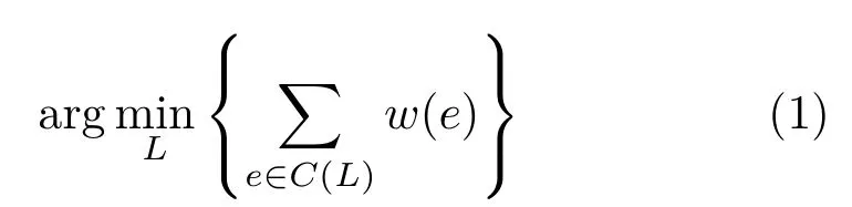
whereC(L)is the set of cut edges associated with the labelingL:

What sets CC apart from other popular clustering problems,such as normalized cuts andk-means clustering,is that the solution of CC automatically recovers the number of optimal clusters.Note that the cutC(L)necessarilyincludes as many negatively weighted edges and as few positively weighted edges as possible.This prevents the result from degenerating to a single cluster(as such a cut uses no negative edges)or|V|clusters(as such a cut includes all positive edges).CC has found uses in problems involving unknown and possibly large number of clusters,such as entity deduplication[37], community detection in social networks[38],gene clustering[39],and image segmentation[10,40–43].
To formulate a clustering problem in terms of CC, the key challenge is designing edge weights.For image segmentation,impressive results have been obtained by weights defined by the local image intensity and learned from a database of ground truth annotations[44].Keuper et al.[10]formulatedpart-basedmesh segmentation in terms of CC.Their weights are built upon primarily part-aware shape descriptors,such as the shape diameter function and dihedral angles.In this paper,we propose a new set of weights tailored forpatch-basedsegmentation, guided by feature lines.
Solving CC is NP-hard[9].Approximate solvers either solve a sequence of linear programs[9,45]or make greedy changes to an initialclustering[10,46–48].The latter seems to have the best efficiency at present for large and sparse graphs[10].Further acceleration by parallelization has also been explored[49,50].However,we have found that even the fastest(serial)CC solver cannot run at interactive speed on our graphs(taking over 10 s for a mesh with 200k faces).Interactive response is critical if we want users to be able to quickly explore diff erent parameter values or perform local edits on the segmentation.In this paper,we show that existing CC solvers can be made much faster, with little loss in optimality,by running on an oversegmentation ofthe mesh pre-computed from the feature lines.
3 Method
3.1 Overview
We consider a triangular mesh(with or without boundary)and a given set of ridge and valley lines on the mesh.Our goal is to connect salient ridges and valleys with shape-following paths to yield a segmentation of the mesh.
A variety of methods exist to compute ridge and valley lines.We use the method of Yoshizawa et al.[51]due to its robustness.Like many other feature line algorithms,each feature line produced by Yoshizawa et al.’s method is represented byfeature pointslying on triangle edges that are connected byfeature segmentsinside triangles.We call those triangle edges that contain feature pointsfeature edges.See Fig.2(a).
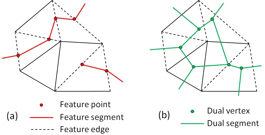
Fig.2 Naming for(a)feature lines and(b)the dual structure.
To formulate the segmentation problem in terms of graph labeling,we have the options of either labeling the triangles or labeling the vertices.Since the feature lines cut across triangles and edges, vertex labeling is a natural choice in our setting. We arrive at the following graph formulation of our problem:given a graphGwhose nodesVand edgesEare respectively the mesh vertices and edges,find a vertex labelingLwhose cutC(L)(defined in Eq.(2)) uses as many salient feature edges and as few other edges(i.e.,weak feature edges and non-feature edges) as possible.This closely resembles the objective of CC mentioned earlier,which is to maximize negative edges and minimize positive edges on the cut.
Our method proceeds in three steps as illustrated in Fig.3:
•Define suitable edge weightswonG(see Fig.3(b)).
•Solve CC onGgiving a vertex labelingL.The initialpatch boundaries are formed by the dualof the cut edges associated withL(see Fig.3(c)).
•Smooth the patch boundaries(see Fig.3(d)).
We next detailthe first and second steps,which are our novelcontributions.The third step is commonly used to post-process segmentations.We use the iterative energy minimization method of Ref.[6], but other smoothing strategies such as the one in Ref.[34]can also achieve visually similar results.
3.2 Defining the weights
To cast our problem in terms of CC,we need to determine weights on the graph edges such that:
•Salient feature edges have negative weights;the more salient the feature,the more negative the edge weight should be.
•Non-salient feature edges,as well as non-feature edges,have positive weights;the more likely that the two vertices connected by the edge belong to the same patch,the more positive the edge weight should be.
To consistently define positive and negative weights that meet the two criteria above,we set the weightw(e)of every edgee∈Eto

Here,Similarity(e)is a positive scalar that measures the likelihood that the two vertices connected byebelong to the same patch.Note that we use the same quantity to measure thesaliencyof a feature edge:the lower Similarity(e),the more salient the feature line cutting across the edgeeis.Award(e)is a positive scalar used to create negative weights for feature edges,and the negativity is controlled by a per-edge parameterαe.We setαe=0 for all nonfeature edgeseto enforce positivity ofw(e).In the automatic mode of our algorithm,we setαe=αfor allfeature edgeewhereαis a user-defined constant.In an interactive session,the user can modify this parameter for individual edges to achieve localized edits(see Section 5).

Fig.3 Main steps of our algorithm.(a)A torus mesh and feature lines(blue)made up of segments interior to triangles.(b)The weighted graph,where negative weights are colored from light blue(small magnitude)to dark blue(large magnitude)and positive weights are colored from light yellow(small magnitude)to red(large magnitude).(c)CC result,with patch boundaries given by the dual segments to the cut edges.(d)Smoothed patched boundaries.
Our definition of the two measures,Similarity and Award,is inspired by recent work on interactive segmentation based on anisotropic geodesic paths[52].The key observation there is that a good segmentation boundary often goes through an anisotropic region(where the minimum and maximum curvature magnitudes differ significantly)andfollows the minimum curvature direction.The authors introduced ananisotropic metricunder which curves appear shorter when they are better aligned with the minimum curvature directions and traveling through more anisotropic regions.
We use a similar anisotropic metric and set Similarity(e)to be the length of adual segmentof edgeeunder this metric.Intuitively,a dualsegment represents a piece of the potential segmentation boundary between the two end vertices ofe.The shorter the dual segment in the anisotropic metric, the more likely that the two vertices ofecan be separated by a good segmentation boundary,and hence the lower Similarity(e).Award(e)is simply set as the length of the dual segment under the regular Euclidean metric.In short,w(e)is theweighted diff erence between the length of the dual segment of e in the anisotropic metric and the Euclidean metric.The two measures,Similarity and Award, are visualized on the Rocker-arm model in Fig.4 (left).Observe that the former gives notably low values near salient features,while the latter merely reflects the Euclidean length of the dual segments of the edges.
We now define in detail Similarity and Award. For completeness,we briefly review the anisotropic metric in Ref.[52].Given a smooth surfaceS,a metric can be represented as a symmetric 2×2 tensorMxat each pointx∈S.The length of a tangent vectorvatxin this metric is
The maximum(minimum)value ofdMx(v)iswhereλ1≥λ2are the eigenvalues ofMx;they are realized whenvis aligned with the corresponding eigenvectore1(e2).As a special case,the standard Euclidean metric is achieved by settingMxto an identity matrix.Letκ1,κ2be the maximum and minimum curvatures atx,such that‖κ1‖≥‖κ2‖,andu1,u2be the corresponding curvature directions.The anisotropic metric in Ref.[52]is represented by a tensorMxwhose eigenvectors{e1,e2}are aligned with{u1,u2}and whose eigenvalues are

wheresx=‖κ1‖−‖κ2‖andγis a global constant.
Recall that our edge weight is the difference between the lengths in the anisotropic metric and the Euclidean metric.To make the two quantities comparable,we modify the metric of Ref.[52]so that the maximal length of a tangent vectorvin the anisotropic metric,is upper bounded by the length ofvin the Euclidean metric,‖v‖.As in Ref.[52],the eigenvectors{e1,e2}of our tensorMxare aligned with{u1,u2},but its eigenvalues become:
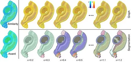
Fig.4 Left:the two measures,Similarity and Award,on all edges.Right-top:the edge weights,w,as the diff erence between Similarity andα∗Award with increasing values ofα.Right-bottom:the corresponding results of CC(after boundary smoothing).
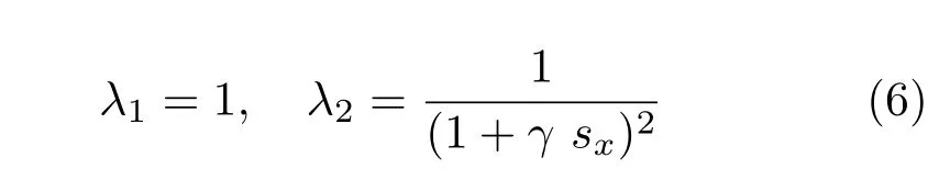
We useγ=0.05 in all our experiments.
Given a discrete mesh,we define a per-triangle anisotropic tensor from locally estimated curvature and curve directions.We create adual vertexfor each triangle located at the triangle centroid,ifnone ofthe three edges is a feature edge,or at the centroid of the feature points otherwise.Thedual segmentof a triangle edgeeis a straight segment connecting two dual vertices.This dual structure is illustrated in Fig.2(b).We evaluate Similarity(e)as the length of the dual segment ofein the anisotropic metric and Award(e)as the length in the Euclidean metric. This is done by first projecting the dual segment onto the supporting plane ofeach ofthe two triangles sharingeand then taking the average of the lengths evaluated in the chosen metric on those triangles (using Eq.(4)).
The global constantα,to whichαeis set in Eq.(3)for all feature edges,controls the negativity of the graph weightw,which in turn governs the granularity of the segmentation.This is the only global parameter in our formulation.Figure 4 visualizes the graph weight for increasing values ofα(top)and the results of CC(bottom).Observe that as the number of negatively weighted edges and the magnitude of their weights increase,the segmentation becomes more refined.Also note that there is a fairly wide range ofαvalues in this example(from 0.5 to 1.1)for which the resulting segmentations appear similar and plausible.The same observation can be made in many of our test examples.
3.3 Solving CC
Efficiently solving CC on large graphs remains a challenging task.Drawing inspirations from applications of CC in image segmentation[10,40–42],our method solves CC on a much smaller,precomputed graph that stillcaptures the essence ofthe input mesh and features.
The basic idea is to first define an initial labelingL′of the original graphG,and then solve CC on a simplified graphG′created by merging vertices ofGwith the same label.The weight of an edge connecting two nodes,sandt,ofG′is the sum of the weights of those edges inGconnecting two nodes that are merged respectively intosandt. Intuitively,vertices and edges ofG′represent the patches and boundaries in an oversegmentation of the mesh.Solving CC onG′yields a labelingLon the original graphG,which eff ectively merges smaller patches of the oversegmentation into bigger patches.
While this is similar to the bottom-up clustering strategy commonly seen in mesh segmentation[11],the key diff erence is that CC is non-parametric.As a result,the merging process requires no ad-hoc termination criteria of the kind needed in previous clustering-based segmentation methods,such as the number of clusters,the area of the patches, thresholds on the segmentation energy,etc.
The key challenge is to find an initial labelingL′so that the induced graphG′is simple enough on one hand,and on the other hand,the resulting labelingLis as close as possible to that obtained by running CC directly on the original graphG.The latter requiresL′to assign different labels to two vertices if they are likely to belong to different patches in the desired segmentation.A conservative approach would be to askallfeature edges to be included in the cut edges associated withL′.Intuitively,we seek an oversegmentation that includes all input feature lines as patch boundaries.
Our method for computing the oversegmentation builds upon previous works[7,36],which extract the watershed of the geodesic distance function from the feature lines.This approach is simple and fast. Moreover,the watershed can effectively bridge the gap between nearby feature lines.However,due to the nature of geodesic distance propagation,the watershed may fail to bridge feature lines that are further apart.Such failure,in turn,results in suboptimal final labelingLafter running CC on the simplified graphG′.An example is given in Fig.5: the watershed(b)fails to connect two ridge lines on a curved ridge that are separated by a long gap(a), as the close-up views highlight.As a result,the final segmentation misses a portion of the ridge(c).
To create an oversegmentation that better connects features,we replace the geodesic distance field by theanisotropicdistance measured in our anisotropic metric(see previous section).Intuitively, distance propagates more slowly along more salient features in the anisotropic metric,which allows the watershed to connect far-apart feature lines as if they were near-by(see Fig.5(d)).Compared with the geodesic watershed[7,36],computing CC on our anisotropic watershed results in not only qualitatively better boundaries(see Fig.5(e))but also lower cut costs(see the quantitative analysis in Section 5).The latter are due to the fact that the anisotropic distance field is propagated using precisely the edge weightswdefined in the original graphG(Eq.(3)),which allows the watershed to naturally cut through graph edges with lower weights.
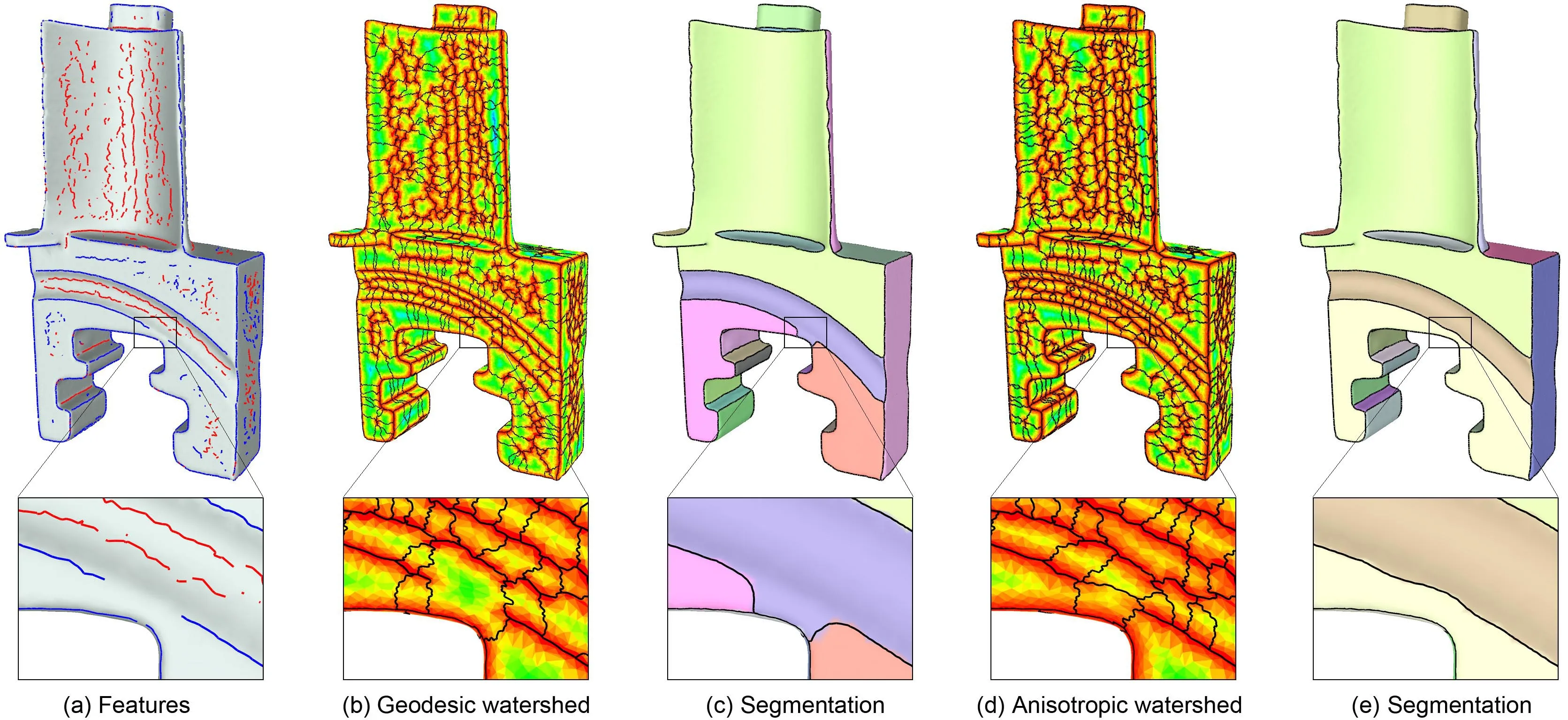
Fig.5 Comparison of(b)the geodesic distance function and(d)our anisotropic distance function,overlayed by their watersheds,from an initial set of feature lines(a).The final segmentations computed by running CC on the respective watersheds are shown(after boundary smoothing)in(c)and(e).Note in the close-up views that segmentation using the geodesic watershed fails to bridge two ridge features,which are connected in the segmentation using our anisotropic watershed.
We now detail the oversegmentation process. To perform distance propagation and extract the watershed,we consider the same dual graph of the triangles as that used for defining the edge weights inG(see Fig.2(b)).Each dualsegment ofa triangleedgeeis assigned the length Similarity(e)(see previous subsection).To start distance propagation, we assign a value of zero to the dual vertex of any triangle that contains some feature edge.The value at any other dual vertex is the shortest distance on the dual graph to any zero-valued dual vertices. We then negate all distance values at the dual vertices and compute the watershed on the dual graph using the immersion algorithm from Ref.[53]. The result is a labeling of dualvertices(and in turn, their corresponding triangles)as eitherwatershedor belonging to a particularbasin.Finally,we label each triangle vertex using the majority label of the basin triangles in its 1-ring neighborhood.
Note that the oversegmentation,and in turn the simplified graphG′,need only to be computed once for a given mesh and feature set.Changing the parameterαein our graph weight definition only affects the edge weighting onG′.This is the key that allows our algorithm to offer rapid feedback during interactive editing.
4 Interaction
Segmentation is an inherently subjective task: the criteria for a good segmentation are highly dependent on both the user and the target application.A key benefit of our CC formulation is that,by modifying the edge weights in the graph,the user has direct and local control of the segmentation result.To free the user from the tedious task of manipulating edge weights,we have developed several intuitive interactions that allow the user to change the granularity of segmentation (globally or locally)and fine-tune the segmentation boundaries.Thanks to our fast CC algorithm,most of these interactions offer interactive response time (i.e.,tens of milliseconds).The only exception is feature sketching,which requires re-computing the oversegmentation.
4.1 Global refinement/coarsening
Recall that,by default,αe=0 for all non-feature edgeseandαe=αfor allfeature edges;αis a global constant.Increasing or decreasingαresults in a finer or coarser segmentation for the entire model.
4.2 Local refinement/coarsening
The user can select a region-of-interest(ROI) and increment or decrement the parameterαefor all edges within that ROI.This results in local refinement or coarsening of the segmentation.Two such edits are illustrated on the Moaimodelin Fig.6. They result in a finer segmentation on the face but a coarser one on the body.
4.3 Feature sketching
The user may sketch over the surface to indicate an intended boundary.This is useful when the desired boundary does not lie on a salient feature.For example,the“cross”-shaped sketch in Fig.7(b)lies in a rather flat region that has no feature lines.We add all triangle edges that intersect the user sketch to the set of feature edges.These newly added feature edges are associated with a largeαe(we use 1.0)to ensure their inclusion in the segmentation. For efficiency,we only update the oversegmentation within those patches in the current segmentation that contain the sketch.

Fig.6 Interactively refinement(from(b)to(c))and coarsening (from(c)to(d))of the segmentation.The user-selected regions are shown in gray in(b)and(c,top),and their updated segmentations are outlined in(c)and(d,top).The corresponding graph weights are shown at the bottom.Note that a refinement operation(increasingαe)results in increased negativity offeature edges(c,bottom),while coarsening(decreasingαe)results in increased positivity(d,bottom).
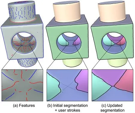
Fig.7 Sketching new feature curves(b,bottom)in a featureless region(a,bottom)results in modified segmentation boundaries(c).
5 Results
Here we perform both quantitative and qualitative analysis of our method.All results in this section are produced automatically without user interaction (other than specifying the global parameterα).As mentioned earlier,we use Ref.[51]to obtain the ridge and valley lines as input to our method.To compute CC on the watershed oversegmentation,we employ the lifted multi-cut method(LMP)[10]which is currently the fastest serial solver on large sparse graphs.We use their GAEC+KLj option without adding long-range edges to the graph.
5.1 Evaluation of CC solver
We first compare the performance of computing CC on the original mesh graphGversus computing it on the simplified graphG′from the watershed oversegmentation.We took the hard disk model (see the bottom of Fig.10),which contains roughly 200k triangles,and explored a range ofαvalues. As shown in Fig.8(top),while running LMP on the original graph can take over 10 s for someαvalues(red curve),running the same solver on the oversegmentation,including the time for computing the oversegmentation,takes about 1 s for allαvalues(cyan curve).More importantly,the time taken to only run LMP,given a pre-computed oversegmentation,is merely tens of milliseconds (magenta curve).All experiments were performed on a PC with a 3.7 GHz CPU and 16 GB ofmemory.
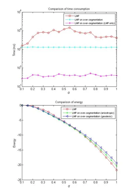
Fig.8 Runtime(top)and cut cost(bottom)for the hard disk model, as a function ofα.
We next evaluate the loss in segmentation quality incurred by our speed-up.To do so,we examine the cut cost,measured by the total weights of the cut edges(Eq.(1)),by running LMP on the original graph,on the watershed oversegmentation based on geodesic distances[7,36],and on our anisotropic watershed.As shown in Fig.8(bottom),the cut cost of the three variants are similar across all values ofα,which validates the use of our speed-up strategy.Furthermore,note that the cut cost using our anisotropic watershed is constantly lower than that using the geodesic watershed[7,36].
5.2 Sensitivity to input
Unlike previous segmentation methods that also utilize feature lines[7,8,36],our method requires no pruning offeatures.Instead,selection and connection of features are handled simultaneously in the CC formulation.Our method is rather insensitive tothe input set of feature lines,whether it has been pruned or not(see Fig.9(left)).The overallstructure of the segmentation remains stable even after the shape is contaminated by noise,which results in a significantly different set of feature lines(see Fig.9(right)).
5.3 Comparisons and examples
We next compare our method with other patchbased segmentations using more examples,in Fig.10. As observed earlier in Fig.1,primitive-fitting[5] and region-growing[6]tend to create additional boundaries in featureless regions where there is large fitting error or variation in curvature.On the other hand,prominent feature lines lying in homogeneous regions may be ignored.In contrast,our method excels at preserving the salient features while avoiding adding non-feature boundaries.Although both our method and that of Mitani and Suzuki[7] work by merging a watershed oversegmentation,ours is guided by the CC formulation which has only one parameter.On the other hand,Mitani and Suzuki use a heuristic merging process with an area-based termination criterion.Even with our best efforts to tune this termination criterion,their method produces much less satisfactory results:the segmentations tend to miss important,fine features and include many weak feature lines in the patch boundaries.
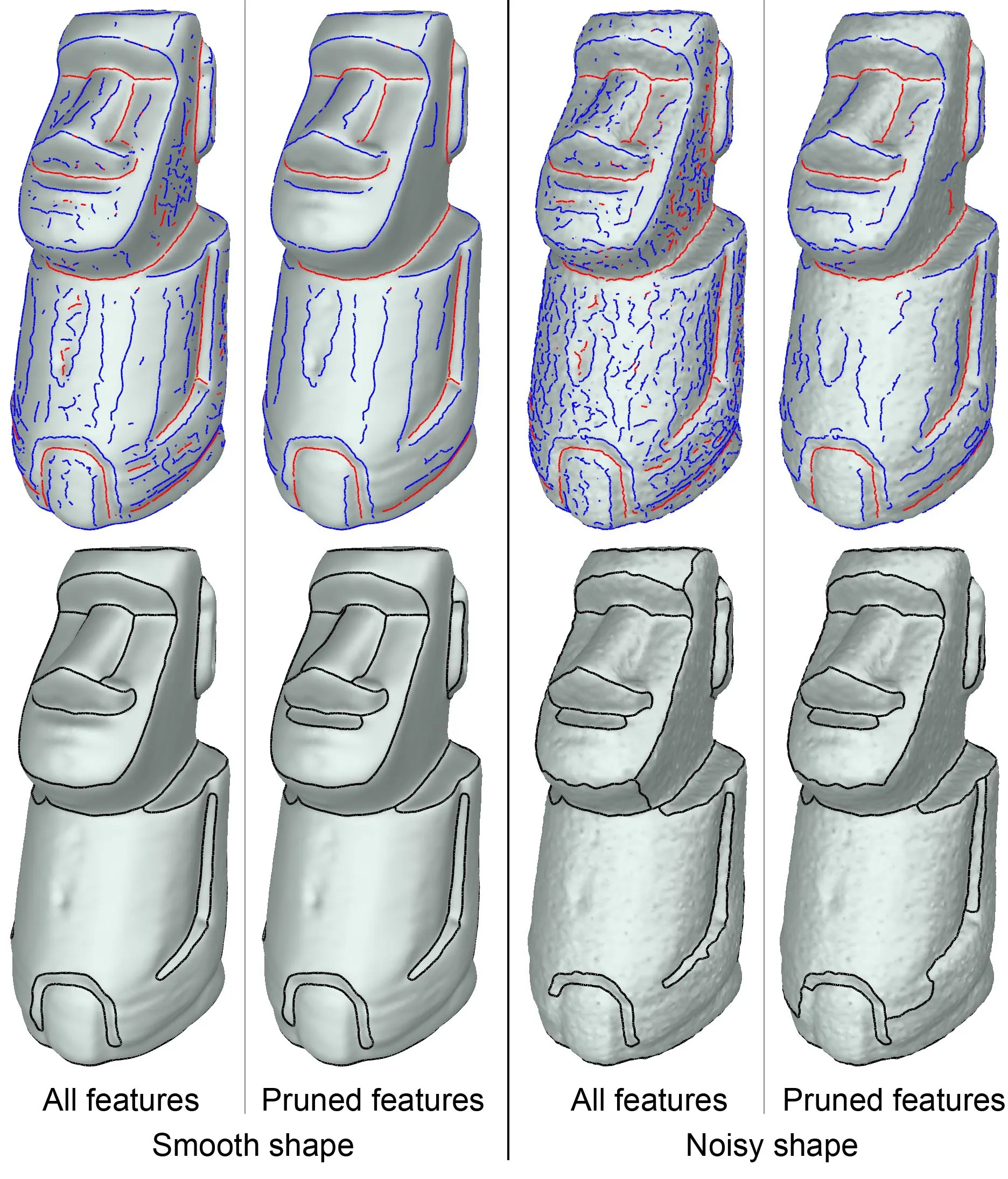
Fig.9 Comparing segmentation results of our method(bottom) given diff erent input sets of feature lines(top)on the original and perturbed shapes.
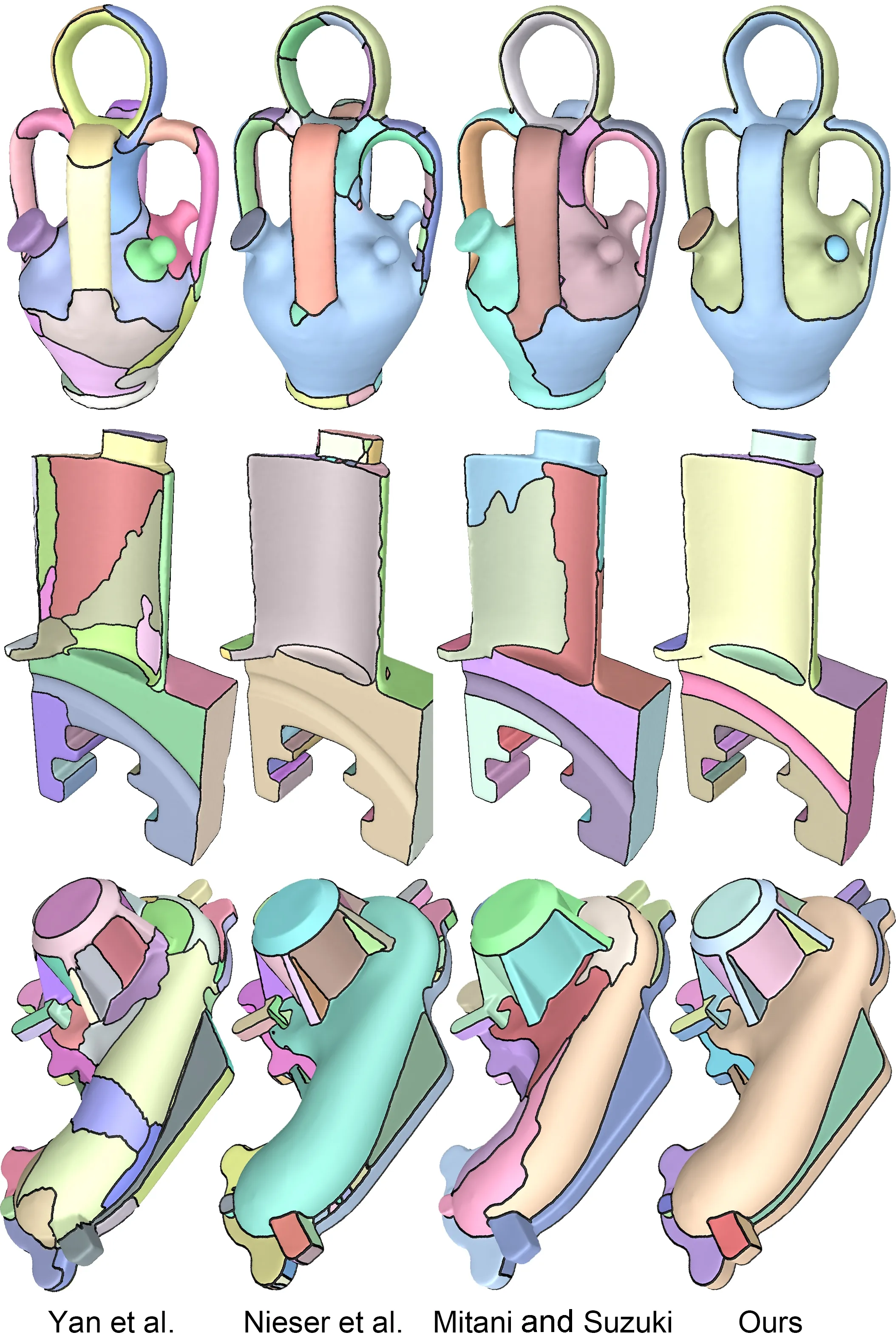
Fig.10 Comparison of the primitive-fitting method of Yan et al.[5], the region-growing method of Nieser et al.[6],the feature-guided method of Mitaniand Suzuki[7],and our method,on three examples.
Finally,we showcase a variety of examples in Fig.11,obtained by our automatic method.Note that these results were all obtained using values ofαwithin a small range(0.5 to 1.0).Please refer to the accompanying video in the Electronic Supplementary Material for 3D views of these results.
6 Limitations and conclusions
6.1 Limitations
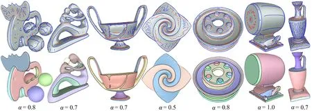
Fig.11 Further segmentation results of our method,showing feature lines(top)and patches(bottom).
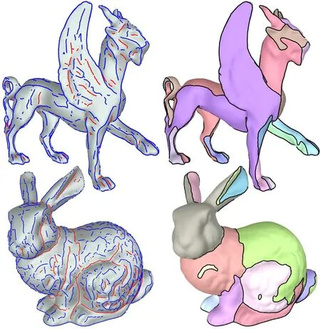
Fig.12 Results of our method on two organic shapes.
Our method is suited to objects that are wellrepresented by their ridge and valley lines.It may not produce meaningful results for organic shapes, whose semantics are primarily captured bypartsinstead ofpatches(two examples are shown in Fig.12).For these shapes,part-based segmentations would be more suitable.Our method considers only the property of the segmentation boundary(i.e., feature saliency).It would be interesting to explore how information from the patch interior,such as regularity ofcurvature and fitting error ofprimitives, could be incorporated into our method.Another interesting question is whether global constraints, such as symmetry,can be added to our formulation to produce more pleasing results.
6.2 Conclusions
We have presented a novel method for segmenting a mesh into patches whose boundaries are aligned with salient features.By formulating the problem in terms of correlation clustering,a non-parametric graph partitioning problem,our method is simple to implement,easy to tune(with a single global parameter),efficient to interact with,and more effective than previous methods in producing feature-aligned segmentations.
Acknowledgements
We thank Dongming Yan for providing the code from Ref.[5]for comparison.The models in this paper were obtained from AIM@SHAPE and Princeton Segmentation Benchmark.The work was supported in part by a gift from Adobe System,Inc.
Electronic Supplementary Material Supplementary material is available in the online version of this article at http://dx.doi.org/10.1007/s41095-016-0071-3.
[1]Cole,F.;Sanik,K.;DeCarlo,D.;Finkelstein,A.; Funkhouser,T.;Rusinkiewicz,S.;Singh,M.How well do line drawings depict shape?ACM Transactions on GraphicsVol.28,No.3,Article No.28,2009.
[2]Mehra,R.;Zhou,Q.;Long,J.;Sheff er,A.;Gooch, A.A.;Mitra,N.J.Abstraction of man-made shapes.ACM Transactions on GraphicsVol.28,No.5,Article No.137,2009.
[3]Gehre,A.;Lim,I.;Kobbelt,L.Adapting feature curve networks to a prescribed scale.Computer Graphics ForumVol.35,No.2,319–330,2016.
[4]Gal,R.;Sorkine,O.;Mitra,N.J.;Cohen-Or, D.iWIRES:An analyze-and-edit approach to shape manipulation.ACM Transactions on GraphicsVol.28, No.3,Article No.33,2009.
[5]Yan,D.-M.;Wang,W.;Liu,Y.;Yang,Z.Variational mesh segmentation via quadric surface fitting.Computer-Aided DesignVol.44,No.11,1072–1082,2012.
[6]Nieser,M.;Schulz,C.;Polthier,K.Patch layout from feature graphs.Computer-Aided DesignVol.42,No.3, 213–220,2010.
[7]Mitani,J.;Suzuki,H.Making papercraft toys from meshes using strip-based approximate unfolding.ACM Transactions on GraphicsVol.23,No.3,259–263, 2004.
[8]Cao,Y.;Yan,D.-M.;Wonka,P.Patch layout generation by detecting feature networks.Computers &GraphicsVol.46,275–282,2015.
[9]Bansal,N.;Blum,A.;Chawla,S.Correlation clustering.Machine LearningVol.56,No.1,89–113, 2004.
[10]Keuper,M.;Levinkov,E.;Bonneel,N.;Lavoue,G.; Brox,T.;Andres,B.Efficient decomposition of image and mesh graphs by lifted multicuts.In:Proceedings of the IEEE International Conference on Computer Vision,1751–1759,2015.
[11]Shamir,A.A survey on mesh segmentation techniques.Computer Graphics ForumVol.27,No.6,1539–1556, 2008.
[12]Attene,M.;Katz,S.;Mortara,M.;Patane,G.; Spagnuolo,M.;Tal,A.Mesh segmentation—A comparative study.In:Proceedings of the IEEE International Conference on Shape Modeling and Applications,7,2006.
[13]Katz,S.;Tal,A.Hierarchical mesh decomposition using fuzzy clustering and cuts.ACM Transactions on GraphicsVol.22,No.3,954–961,2003.
[14]Au,O.K.-C.;Zheng,Y.;Chen,M.;Xu,P.;Tai,C.-L. Mesh segmentation with concavity-aware fields.IEEE Transactions on Visualization and Computer GraphicsVol.18,No.7,1125–1134,2012.
[15]Lien,J.-M.;Amato,N.M.Approximate convex decomposition of polyhedra and its applications.Computer Aided Geometric DesignVol.25,No.7,503–522,2008.
[16]Asafi,S.;Goren,A.;Cohen-Or,D.Weak convex decomposition by lines-of-sight.Computer Graphics ForumVol.32,No.5,23–31,2013.
[17]Fan,R.;Jin,X.;Wang,C.C.L.Multiregion segmentation based on compact shape prior.IEEE Transactions on Automation Science and EngineeringVol.12,No.3,1047–1058,2015.
[18]Shapira,L.;Shamir,A.;Cohen-Or,D.Consistent mesh partitioning and skeletonisation using the shape diameter function.The Visual ComputerVol.24,No. 4,249–259,2008.
[19]Zhang,H.;Liu,R.Mesh segmentation via recursive and visually salient spectral cuts.In:Proceedings of Vision,Modeling,and Visualization,429–436,2005.
[20]Lee,Y.;Lee,S.;Shamir,A.;Cohen-Or,D.;Seidel,H.-P.Mesh scissoring with minima rule and part salience.Computer Aided Geometric DesignVol.22,No.5,444–465,2005.
[21]Kalogerakis,E.;Hertzmann,A.;Singh,K. Learning 3D mesh segmentation and labeling.ACM Transactions on GraphicsVol.29,No.4,Article No.102,2010.
[22]Cohen-Steiner,D.;Alliez,P.;Desbrun,M.Variational shape approximation.ACM Transactions on GraphicsVol.23,No.3,905–914,2004.
[23]Wu,J.;Kobbelt,L.Structure recovery via hybrid variationalsurface approximation.Computer Graphics ForumVol.24,No.3,277–284,2005.
[24]Attene,M.;Falcidieno,B.;Spagnuolo,M.Hierarchical mesh segmentation based on fitting primitives.The Visual ComputerVol.22,No.3,181–193,2006.
[25]Zhang,H.;Li,C.;Gao,L.;Wang,G.Hierarchical mesh segmentation based on quadric surface fitting. In:Proceedings of the 14th International Conference on Computer-Aided Design and Computer Graphics (CAD/Graphics),33–40,2015.
[26]Julius,D.;Kraevoy,V.;Sheff er,A.D-charts:Quasidevelopablemesh segmentation.Computer Graphics ForumVol.24,No.3,581–590,2005.
[27]Wang,C.Computing length-preserved free boundary for quasi-developable mesh segmentation.IEEE Transactions on Visualization and Computer GraphicsVol.14,No.1,25–36,2008.
[28]Mangan,A.P.;Whitaker,R.T.Partitioning 3D surface meshes using watershed segmentation.IEEE Transactions on Visualization and Computer GraphicsVol.5,No.4,308–321,1999.
[29]Sun,Y.;Paik,J.K.;Koschan,A.F.;Page,D. L.;Abidi,M.A.Triangle mesh-based edge detection and its application to surface segmentation and adaptive surface smoothing.In:Proceedings of the International Conference on Image Processing,Vol.3, 825–828,2002.
[30]Razdan,A.;Bae,M.A hybrid approach to feature segmentation of triangle meshes.Computer-Aided DesignVol.35,No.9,783–789,2003.
[31]Lavoue,G.;Dupont,F.;Baskurt,A.A new CAD mesh segmentation method,based on curvature tensor analysis.Computer-Aided DesignVol.37,No.10,975–987,2005.
[32]Kim,H.S.;Choi,H.K.;Lee,K.H.Feature detection of triangular meshes based on tensor voting theory.Computer-Aided DesignVol.41,No.1,47–58,2009.
[33]Gelfand,N.;Guibas,L.J.Shape segmentation using local slippage analysis.In:Proceedings of the Eurographics/ACM SIGGRAPH Symposium on Geometry Processing,214–223,2004.
[34]Lai,Y.-K.;Hu,S.-M.;Martin,R.R.;Rosin,P.L. Rapid and effective segmentation of 3D models using random walks.Computer Aided Geometric DesignVol. 26,No.6,665–679,2008.
[35]Wang,S.;Hou,T.;Li,S.;Su,Z.;Qin,H. Anisotropic elliptic PDEs for feature classification.IEEE Transactions on Visualization and Computer GraphicsVol.19,No.10,1606–1618,2013.
[36]L´evy,B.;Petitjean,S.;Ray,N.;Maillot,J.Least squares conformal maps for automatic texture atlasgeneration.ACM Transactions on GraphicsVol.21, No.3,362–371,2002.
[37]Arasu,A.;R´e,C.;Suciu,D.Large-scale deduplication with constraints using dedupalog.In:Proceedings of the IEEE 25th International Conference on Data Engineering,952–963,2009.
[38]Yang,B.;Cheung,W.K.;Liu,J.Community mining from signed social networks.IEEE Transactions on Know ledge and Data EngineeringVol.19,No.10, 1333–1348,2007.
[39]Ben-Dor,A.;Shamir,R.;Yakhin,Z.Clustering gene expression patterns.Journal of Computational BiologyVol.6,Nos.3–4,281–297,2004.
[40]Kim,S.;Nowozin,S.;Kohli,P.;Yoo,C.D.Higherorder correlation clustering for image segmentation. In:Proceedings of Advances in Neural Information Processing Systems,1530–1538,2011.
[41]Yarkony,J.;Ihler,A.T.;Fowlkes,C.C.Fast planar correlation clustering for image segmentation. In:Computer Vision–ECCV 2012.Fitzgibbon,A.; Lazebnik,S.;Perona,P.;Sato,Y.;Schmid,C.Eds. Springer Berlin Heidelberg,568–581,2012.
[42]Beier,T.;Kroger,T.;Kappes,J.H.;Kothe, U.;Hamprecht,F.A.Cut,glue,&cut:A fast, approximate solver for multicut partitioning.In: Proceedings of the IEEE Conference on Computer Vision and Pattern Recognition,73–80,2014.
[43]Kappes,J.H.;Swoboda,P.;Savchynskyy,B.;Hazan, T.;Schn¨orr,C.Probabilistic correlation clustering and image partitioning using perturbed multicuts.In:Scale Space and Variational Methods in Computer Vision.Aujol,J.-F.;Nikolova,M.;Papadakis,N.Eds. Springer International Publishing,231–242,2015.
[44]Arbelaez,P.;Maire,M.;Fowlkes,C.;Malik, J.Contour detection and hierarchical image segmentation.IEEE Transactions on Pattern Analysis and Machine IntelligenceVol.33,No.5, 898–916,2011.
[45]Demaine,E.D.;Emanuel,D.;Fiat,A.;Immorlica, N.Correlation clustering in general weighted graphs.Theoretical Computer ScienceVol.361,Nos.2–3,172–187,2006.
[46]Ailon,N.;Charikar,M.;Newman,A.Aggregating inconsistent information:Ranking and clustering.Journal of the ACMVol.55,No.5,Article No.23, 2008.
[47]Bagon,S.;Galun,M.Large scale correlation clustering optimization.arXiv preprintarXiv:1112.2903,2011.
[48]Lingas,A.;Persson,M.;Sledneu,D.Iterative merging heuristics for correlation clustering.International Journal of MetaheuristicsVol.3,No.2,105–117,2014.
[49]Chierichetti,F.;Dalvi,N.;Kumar,R.Correlation clustering in MapReduce.In:Proceedings of the 20th ACM SIGKDD International Conference on Knowledge Discovery and Data Mining,641–650, 2014.
[50]Pan,X.;Papailiopoulos,D.S.;Oymak,S.;Recht,B.; Ramchandran,K.;Jordan,M.I.Parallel correlation clustering on big graphs.In:Proceedings of Advances in Neural Information Processing Systems,82–90, 2015.
[51]Yoshizawa,S.;Belyaev,A.;Seidel,H.-P.Fast and robust detection of crest lines on meshes.In: Proceedings of the ACM Symposium on Solid and Physical Modeling,227–232,2005.
[52]Zhuang,Y.;Zou,M.;Carr,N.;Ju,T.Anisotropic geodesics for live-wire mesh segmentation.Computer Graphics ForumVol.33,No.7,111–120,2014.
[53]Vincent,L.;Soille,P.Watersheds in digital spaces: An efficient algorithm based on immersion simulations.IEEE Transactions on Pattern Analysis and Machine IntelligenceVol.13,No.6,583–598,1991.

Yixin Zhuang is an assistant researcher in the National Digital Switching System Engineering& Technological Research Center,China. He obtained his B.S.degree from Nanjing University of Aeronautics and Astronautics in 2008,and both M.S. and Ph.D.degrees from the National University of Defense Technology in 2011 and 2015, respectively.His research interests include computer graphics,and geometric modeling and processing.

Hang Dou studied computer science as an undergraduate in Zhejiang University,China,where he received his B.A.degree in 2010.He received his M.S.degree in computer science from the University of Iowa in 2013. He is currently a Ph.D.student in the Computer Science and Engineering Department in Washington University in St.Louis, USA.His primary research area is computer graphics, with particular interests in mesh processing,shape understanding,and fast rendering.

Nathan Carr is a principal scientist in Adobe Research leading a team of graphics researchers.He obtained his B.S.degree from the College of William &Mary,M.S.degree from Washington State University,and Ph.D.degree from the University of Illinois Urbana-Champaign.Since joining Adobe,he has produced numerous features for Adobe’s flagship products including Photoshop and Illustrator.The technologies span the domains of 3D photorealistic rendering,image processing,geometric modeling,and 3D printing.Nathan has authored dozens of academic papers and continues to guide research and development at Adobe.

Tao Ju is a professor in the Department of Computer Science and Engineering in Washington University in St.Louis, USA.He obtained his B.S.and B.A. degrees from Tsinghua University, China,in 2000,and his Ph.D.degree in computer science from Rice University in 2005.His research interests include computer graphics,geometry processing,and applications to biomedicine.He has received a number of grants from NSF and NIH,including an NSF CAREER Award.He has served as an associate editor forIEEE Transactions on Visualization and Computer Graphics,Computer Graphics Forum,Computer-Aided Design,Graphical Models,andComputational Visual Media.
Open Access The articles published in this journal are distributed under the terms of the Creative Commons Attribution 4.0 International License(http:// creativecommons.org/licenses/by/4.0/),which permits unrestricted use,distribution,and reproduction in any medium,provided you give appropriate credit to the original author(s)and the source,provide a link to the Creative Commons license,and indicate if changes were made.
Other papers from this open access journalare available free of charge from http://www.springer.com/journal/41095. To submit a manuscript,please go to https://www. editorialmanager.com/cvmj.
1 National Digital Switching System Engineering& Technological Research Center,Zhengzhou,450001, China.E-mail:yixin.zhuang@gmail.com
2 Washington University in St.Louis,St.Louis,63130, USA.E-mail:H.Dou,hangdou@gmail.com;T.Ju, taoju@cse.wustl.edu
3 Adobe,San Francisco,94103,USA.E-mail: ncarr@adobe.com.
t
2016-08-24;accepted:2016-12-22
 Computational Visual Media2017年2期
- Computational Visual Media的其它文章
- View suggestion for interactive segmentation of indoor scenes
- Feature-based RGB-D camera pose optimization for real-time 3D reconstruction
- EasySVM:A visual analysis approach for open-box support vector machines
- User-guided line abstraction using coherence and structure analysis
- Fast and accurate surface normal integration on non-rectangular domains
- Robust camera pose estimation by viewpoint classification using deep learning