Fast and accurate surface normal integration on non-rectangular domains

Martin B¨ahr,Michael BreußYvain Qu´eau,Ali SharifiBoroujerdi,and Jean-Denis Durou

Fast and accurate surface normal integration on non-rectangular domains

Martin B¨ahr1,Michael Breuß1Yvain Qu´eau2,Ali SharifiBoroujerdi1,and Jean-Denis Durou3

The integration of surface normals for the purpose of computing the shape of a surface in 3D space is a classic problem in computer vision.However, even nowadays it is still a challenging task to devise a method that is flexible enough to work on non-trivial computationaldomains with high accuracy,robustness, and computational efficiency.By uniting a classic approach for surface normal integration with modern computational techniques,we construct a solver that fulfils these requirements.Building upon the Poisson integration model,we use an iterative Krylov subspace solver as a core step in tackling the task.While such a method can be very efficient,it may only show its full potential when combined with suitable numerical preconditioning and problem-specific initialisation.We perform a thorough numerical study in order to identify an appropriate preconditioner for this purpose. To provide suitable initialisation,we compute this initial state using a recently developed fast marching integrator.Detailed numerical experiments illustrate the benefits of this novel combination.In addition,we show on real-world photometric stereo datasets that the developed numerical framework is flexible enough to tackle modern computer vision applications.

surface normal integration;Poisson integration;conjugate gradient method;preconditioning;fast marching method; Krylov subspace methods;photometric stereo;3D reconstruction

1 Introduction

The integration of surface normals is a fundamental task in computer vision.Classic examples of processes where this technique is often applied are image editing[1],shape from shading as analysed by Horn[2],and photometric stereo(PS) for which we refer to the pioneering work of Woodham[3].Modern applications of PS include facial recognition[4],industrial product quality control[5],object preservation in digitalheritage[6], and new utilities with potential use in the video (game)industry and robotics[7],among many others.

In this paper we consider surface normal integration in the context of the PS problem,which serves as a role model for potential applications. The task of PS is to compute the 3D surface of an object from multiple images ofthe same scene under different illumination conditions.The standard PS method for reconstructing an unknown surface has two stages.In a first step,the surface is represented as a field of surface normals,or equivalently,a corresponding gradient field.In a subsequent step this is integrated to obtain the depth of the surface.

To handle the integration step,many different approaches and methods have been developed during recent decades.However,despite all these developments there is still the need for approaches that combine a highaccuracyreconstruction withrobustnessagainst noise and outliers,and reasonable computationalefficiencyfor working with high-resolution cameras and corresponding imagery.

Computational issues.Let us briefly elaborate on the demands on an idealintegrator.As discussed, e.g.,in Ref.[8],a practical issue is robustness with respect to noise and outliers.Since computer vision processes such as PS rely on simplified assumptions that often do not hold for realistic illumination and surface reflectance,artefacts may often arise when estimating surface normals from real-world input images.Therefore,the determined depth gradient field is not noise-free and may also contain outliers. These may strongly influence the integration process.

Secondly,objects to be reconstructed in 3D are typically in the centre of a photographed scene. Therefore,they only form part of each input image.The sharp gradient usually representing the transition from foreground to background is a difficult feature for most surface normal integrators and generally influences the estimated shape of the object of interest.Because of this it is desirable to consider only image segments that represent the object of interest and not the background.Although similar difficulties(sharp gradients)also arise for discontinuous surfaces that may appear at selfocclusions of an object[9],we do not tackle this issue in the present article.Instead,we neglect self-occlusion and focus on reconstructing asmoothsurface on the(possibly non-rectangular)subset of the image domain representing the object of interest. Related to this point,another important aspect is the computational time and cost saving that can be achieved by the concomitant decrease in the number of elements of the computational domain.For reasons ofboth reconstruction quality and efficiency, an ideal solver for surface normal integration should thus work on non-rectangular domains.

Finally,to capture ever more detail in 3D reconstruction,camera technology evolves and the resolution of images tends to increase continually. This means,the integrator has to work accurately and quickly for various sizes of input images, including images of size at least 1000×1000 pixels. Consequently,the computational efficiency of a solver is a key requirement for many possible modern and future applications.

To summarise,one can identify the desirable properties ofrobustnesswith respect to noise and outliers,ability to work onnon-rectangular domains, andefficiencyof the method:one aims for an accurate solution using reasonable computational resources(such as time and memory).

Related work.Many methods taking into account the abovementioned issues individually have been developed to solve the problem of surface normal integration during recent decades.

According to Klette and Schl¨uns[10],such methods can be classified as local and global integration methods.

The most basic local method,also referred to as direct line-integration scheme[11–13],is based on the line integral technique and the fact that a closed path on a continuous surface should be zero.These methods are in general quite fast, but due to their local nature,the reconstructed solution depends on the integration path.Another more recent local approach for normal integration is based on an eikonal-type equation,which can be solved by applying the computationally efficient fast marching(FM)method[14–16].However,a common disadvantage of all local approaches is sensitivity with regard to noise and discontinuities,which lead to error accumulation in the reconstruction.

In order to minimise error accumulation,it is preferable to adopt a global approach based on the calculus ofvariations.Horn and Brooks[2]proposed the classic and most natural variational method for the intended task by casting the corresponding functional in a form that results in a least-squares approximation.The necessary optimality condition represented by the Euler–Lagrange equation of the classic functional is given by the Poisson equation, which is an elliptic partial differential equation. This approach to surface normal integration is often calledPoisson integration.The practicaltask arising amounts to solving the linear system of equations that corresponds to the discretised Poisson equation.

Direct methods for solving the latter system,as for instance Cholesky factorisation,can be fast,but this type of solver may use a substantial amount of memory and appears to be rather impractical for images oflarger than 1000×1000 pixels.Moreover,if based on matrix factorisation,the factorisation itself is relatively expensive to compute.Generally,direct methods offer an extremely highly accurate result, but one must pay a high computational price.In contrast,iterative methodsare not naturally notedfor extremely high accuracy but are very fast when computing approximate solutions.They require less memory and are thus inherently more attractive candidates for this application,but involve some non-trivial aspects(see later)which make them less straightforward to use.

An alternative approach to solving the leastsquares functional was introduced by Frankot and Chellappa[17].The main idea is to transform the problem to the frequency domain where a solution can be computed in linear time through the fast Fourier transform,if periodic boundary conditions are assumed.The latter unfavourable condition can be resolved by use of the discrete cosine transform(DCT)as shown by Simchony et al.[18].However,these methods remain limited to rectangular domains.To apply these methods on non-rectangular domains requires introducing zeropadding in the gradient field which may lead to an unwanted bias in the solution.Some conceptually related basis function approaches include the use of wavelets[19]and shapelets[20].The method of Frankot and Chelappa was enhanced by Wei and Klette[21]to improve its accuracy and robustness to noise.Another approach was proposed by Kara¸cali and Snyder[22]who make use ofadditionaladaptive smoothing for noise reduction.

Among all of the mentioned global techniques,variational methodsoffer a high robustness with respect to noise and outliers.Therefore,many extensions have been developed in modern works[9, 23–28].Agrawal et al.[23]use anisotropic instead of isotropic weights for the gradients during integration.Durou et al.[9]give a numerical study of several functionals,in particular with nonquadratic and non-convex regularisations.To reduce the influence of outliers,theL1norm has also become an important regularisation instrument[25, 26].In Ref.[24]the extension toLpminimisation with 0＜p＜1 is presented.Two other recent works are Ref.[27]where the use of alternative optimisation schemes is explored and Ref.[28] where the proposed formulation leads to the task of solving a Sylvester equation.Nevertheless,these methods have some drawbacks.By the application of additionalregularisation as in Refs.[9,23–27],depth reconstruction becomes quite time-consuming and the correct setting of parameters is more difficult, while the approach of Harker and O’Leary[28]is only efficient for rectangular domainsΩ.

Summarizing the achievements of previous works, the problem of surface normal integration on nonrectangular domains has not yet been perfectly solved.The main challenge is still to find a balance between quality and time needed to generate the result.One should take into account that to achieve better quality in 3D object reconstruction,the resolution of images tends to increase continually, and so computational efficiency is surely a key requirement for many potential current and future applications.

Our contributions.To balance the aspects of quality,robustness,and computationalefficiency,we go back to the powerful classic approach of Horn and Brooks as the variational framework has the benefit of high modeling flexibility.In detail,our contributions when extending this classic path of research are:

1.Building upon a recent conference paper where we compared several Krylov subspace methods for surface normalintegration[29],we investigate the use of the preconditioned conjugate gradient(PCG)method for performing Poisson integration over non-trivial computational domains.While such methods constitute advanced yet standard methods in numerical computing[30,31],they are not yet standard tools in image processing,computer vision,and graphics.To be more precise,we propose to employ the conjugate gradient(CG) scheme as the iterative solver and we explore modern variations of incomplete Cholesky (IC)decomposition for preconditioning.The thorough numerical investigation here represents a significant extension of our conference paper.

2.For computing a good initialisation for the PCG solver,we employ a recent FM integrator[15] already mentioned above.Its main advantages are its flexibility for use with non-trivialdomains coupled with low computational requirements. While we proposed this means of initialisation already in Ref.[29],our numerical extensions mean that the conclusion we draw in this paper is much sharper.

3.We prove experimentally that our resulting, combined novel method unites the advantages offl exibilityandrobustnessof variational methods withlow computational timeandlow memory requirements.

4.We propose a simple yet effective modification for gradient fields containing severe outliers,for use with Poisson integration methods.

The abovementioned building blocks of our method represent a pragmatic choice among current tools for numerical computing.Moreover,as demonstrated by our new integration model that is specifically designed for tackling data with outliers, our numerical approach can be readily adapted to other Poisson-based integration models.This, together with the well-engineered algorithm for our application,i.e.,FM initialisation and fine-tuned algorithmic parameters,makes our method a unique, efficient,and flexible procedure.

2 Surface normal integration

The mathematical set-up of surface normal integration(SNI)can be described as follows. We assume that for a domainΩ,a normalfieldn:=n(x,y)=[n1(x,y),n2(x,y),n3(x,y)]Tis given for each grid point(x,y)∈Ω.The task is to recover a surfaceS,which can be represented as a depth mapv(x,y)over(x,y)∈Ω,such thatnis the normal field ofv.Assuming orthographic projection①The perspective integration problem can be formulated in a similar way,using the change of variablev=logv[32].,the normalfieldnof a surface at(x,y,v(x,y))∈R3can be written as

withvx:=∂v/∂x,vy:=∂v/∂y,and▽v:=[vx,vy]T. Moreover,the components ofnare given by partial derivatives ofv:

where we think ofpandqas given data.

A detailed description of the fast marching integrator can be found in Refs.[15,16],and the presentation of the components of the CG scheme can be found in literature on Krylov subspace solvers, e.g.,Ref.[31].We still summarize the algorithms in some detail here because there are important parameters that need to be set and some choices to make:since the efficiency of integrators depends largely on such practicalimplementation details,our explanations provide additionalvalue beyond a plain description of the methods.

While our discretisation of the Poisson equation is a standard one,we deal with non-trivial boundary conditions in our application,necessitating a thorough description.The construction of our non-standard numericalboundary conditions,which is often overlooked in the literature,is another technical contribution to the field.

2.1 Fast marching integrator

We recall for the convenience of the reader some relevant developments from Refs.[14–16],which showed that it is possible to tackle the problem of surface normal integration via the following PDE-based model inw=v+λf:

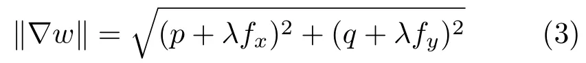
whereλ＞0 andf:R2→R are user-defined.Using PDE(3)we do not compute the depth functionvdirectly,but instead we solve in a first step for a functionw.This means,to obtainvone has to solve the eikonal-type equation forw,in which▽v=(p,q)and▽fare known,and recovervin a second step from the computedwby subtracting the known functionf.The intermediate step of considering a new functionwis necessary for successful application of the FM method,in order to avoid local minima and ensure that any initial point can be considered[14].It turns out that a natural candidate forfis the squared Euclidean distance function with its minimum in the centre of the domain(x0,y0)=(0,0),i.e.,

Other choices forfare also possible[16].As boundary condition we may employw(0,0)=0. After computation ofwwe easily compute the sought depth mapvviav=w−λf.Let us note that the FM integrator requires parameterλto be tuned,but it is not a crucial choice as any large numberλ≫0will work[15]①In our experiments,we used the valueλ=105..

Numerical upwinding.A crucial issue for the FM integrator is correct discretisation of the derivatives offin Eq.(3).In order to obtain a stable method,an upwind discretisation of the partial derivatives offis required:

写之是对意境的表达，“意在笔先”看似老生常谈，实则是画家的普遍经验，“写”看似技法，实则是对“意境”的把握。中国画中“笔墨”非“写之”不能得之，“写意精神”更是中国传统文化的至高追求，“六法”的标准正是对中国传统文化中“写意精神”的最好诠释，也是对中国传统文化中的哲学思想的最好体现。

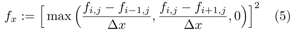
and analogously forfy,for grid widths∆xand∆y.

Making use of the same discretisation for the components of▽w,one obtains a quadratic equation that must be solved for every pixel except at the initial pixel(0,0)where some depth value is prescribed.

Let us note that the initial point can be chosen in practice anywhere,i.e.,there is no restriction to (0,0).

Non-convex domains.If the above method is used without modification over non-convex domains, the FM integrator fails to reconstruct the solution. The reason is that the original,unmodified squared Euclidean distance does not yield a meaningful distance from the starting point to pixels which are not connected by a direct line lying within the integration domain.In other words,the unmodified scheme just works over convex domains.

To overcome the problem,a suitable distance which calculates the shortest path from the starting point to every point on the computationaldomain is necessary.To this end,the use ofa geodesic distance functiondis advocated[15].We proceed as follows, relying on similar ideas to those in,e.g.,Ref.[33]for path planning.In a first step we solve an eikonal equation=1 over allthe points of the domain withd:=0 at the chosen start point.This can of course be done again with the FM method.Then,in a second step we are able to compute the depth mapv.Therefore,we use Eq.(3)forw,with the squared geodesic distance functiondinstead offand using Eq.(5).Afterwards we recovervviav=w−λd.

Fast marching algorithm.The idea of FM goes back to Refs.[34–36].For a comprehensive introduction see Ref.[37].The benefit of FM is its relatively low complexity ofO(nlogn)wherenis the number of points in the computational domain②When using the untidy priority queue structure[38]the complexity may even be lowered toO(n)..

Let us briefly describe the FM strategy.The principle behind FM is that information advances from smaller values ofwto larger values ofw,thus visiting each point ofthe computationaldomain just once.To this end,one may employ three disjoint sets of nodes as discussed in detail in Refs.[37,39]:{s1}accepted nodes,{s2}trial nodes,and{s3}far nodes.The valueswi,jfor set{s1}are considered known and will not be changed.A memberwi,jin set{s2}is always at a neighbour ofan accepted node. This is the set where the computation actually takes place and the values ofwi,jcan still change.Set{s3}contains those nodeswi,jwhere an approximate solution has not yet been computed as these are not in a neighbourhood of a member of{s1}.

The FMalgorithm iterates the following procedure untilall nodes are accepted:

(a)Find the grid pointAin{s2}with the smallest value and move it to{s1}.

(b)Place allneighbours ofAinto{s2}ifnot already there and compute the arrival time for all of them,if they are not already in{s1}.

(c)If the set{s2}is not empty,return to(a).

For initialisation,one may start by putting the node at(0,0)into set{s1};it bears the boundary condition of the PDE(3).

An efficient implementation amounts to storing the nodes in{s2}in a heap data structure,so the smallest element in step(a)can be chosen as quickly as possible.

2.2 Poisson integration

The first part ofthis section is dedicated tomodeling. We first briefly review the classic variational approach to the Poisson integration(PI)problem[2, 18,27,28,32].The handling ofextremely noisy data motivates modifications of the underlying energy functional(6),e.g.,see Ref.[27].By proposing a new modeldealing with outliers,we demonstrate that the Poisson integration framework is flexible enough to dealwith such modern approaches.

The second part is devoted to thenumerics.We propose a dedicated,and somewhat non-standard, discretisation for our application.

Classic Poisson integration model.In order to recover the surface it is common to minimise the least-squares error between the input and the gradient field ofvby minimising:

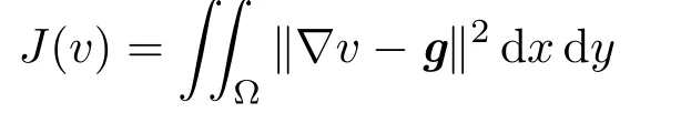
whereg=[p,q]T.

A minimiservof Eq.(6)must satisfy the associated Euler–Lagrange equation which is equivalent to the followingPoisson equation:

that is usually complemented by(natural)Neumann boundary conditions(▽v−g)·µ=0,where the vectorµis normalto∂Ω.In this case,uniqueness of the solution is guaranteed,apart from an additional constant.Thus,one recovers the shape but not absolute depth(as in FM integration).

A modified PDE for normal fields with outliers.We now demonstrate by giving an example that the PI framework is flexible enough to also deal with gradient fields featuring strong outliers.To this end,we propose a simple,yet effective way to modify the PImodelin order to limit the influence of outliers.Other variations for diff erent applications, e.g.,self-occlusions[9,27],are ofcourse also possible.

Let us briefly recall that the classic model in Eq.(6)which leads to the Poisson equation in Eq.(7) is based on a simple least-squares approach.At locations(x,y)corresponding to outliers,the valuesp(x,y)andq(x,y)are not reliable,and one would prefer to limit the influence of such corrupt data.

Therefore,we modify the Poisson equation in Eq.(7)by introducing a space-dependent fidelity termν:=ν(x,y)by

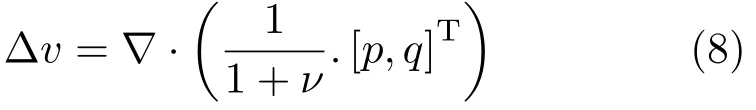
Let us note that a similar strategy,namely to introduce modeling improvements in a PDE that is originally the Euler–Lagrange equation of an energy functional,instead of modifying it,is occasionally employed in computer vision:see,e.g.,Ref.[40]. However,we do not tinker here with the core of the PDE,i.e.,the Laplace operator∆,but merely include preprocessing by modifying the right hand side of the Poisson equation.

The key to effective preprocessing is of course to consider the role ofνso that it smooths the surface only at locations where the input gradient is unreliable.Thus,we seek a functionν(x,y)which is close to zero if the input gradient is reliable,and takes high values if it is not.

Theintegrabilityterm should vanish if the surface isC2-smooth.This argument was used in Ref.[27]to suggest an integrability-based weighted least-squares functional able to recover discontinuity jumps,which generally correspond to a high absolute value of integrability.

Since integrability not only indicates the location of discontinuities,but also that of the outliers,we suggest use ofthis integrability term to find a smooth surface explaining a corrupted gradient.To do so, we use the following choice for our regularisation parameter:

for which the desired properties(i)vanish when integrability is low(reliable gradients),and(ii)take a high value when integrability is high(outliers).

Putting Eqs.(9)and(10)in Eq.(8),our new model amounts to solving the following equation:

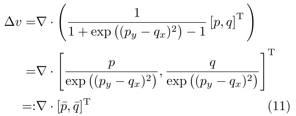
which is another Poisson equation,where the right hand side can be computeda priorifrom the input gradient.

Let us clarify explicitly that the meaning of Eq.(11)is to replace the vector of given data[p,q]Tdescribing the normal field by a modified version [¯p,¯q]Tas defined in Eq.(11).

In addition,we emphasise thatallmethods for SNI based on such a Poisson equation are straightforward to adapt:it suffices to replace(p,q)by.The algorithmic complexity of all of such approaches remains exactly the same.The practical validity of this simple new model and its benefit of better numerics are demonstrated in Section 4.

In the main part of our paper,for simplicity of presentation,we will simply consider the classic model in Eq.(7)and come back to the proposed modification in Section 4.5.

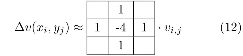
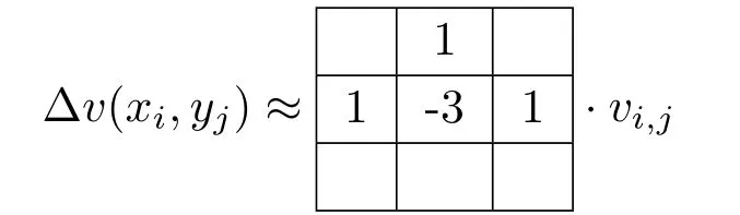
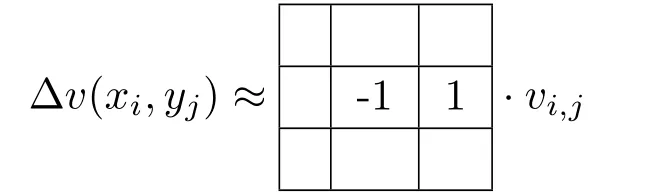
Discretisation of the Poisson equation.A useful standard numerical approach to solving the Poisson PDE as in Eqs.(7)or(11)makes use offinite differences.Often,div(p,q)and∆v=vxx+vyyare approximated by central differences.For simplicity, we suppose that the grid size is∆x=∆y=1 as common practice in image processing.Then,asuitable discrete version of the Laplacian is given in stencilnotation by

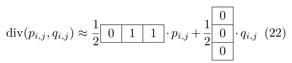
so the divergence is given by

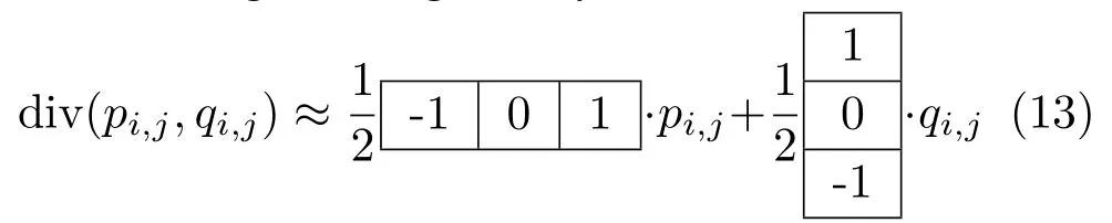
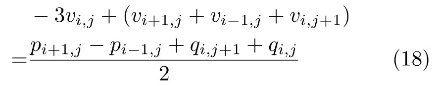
where the measured gradientg=[p,q]T.Making use of Eqs.(12)and(13)to discretize Eq.(7)leads to

which corresponds to a linear systemAx=b,where the vectorsxandbare obtained by stacking the unknown valuesvi,jand the given data,respectively. The matrixAcontains the coefficients arising by discretizing the Laplace operator∆.

We employ in all experiments here the above discretisation,as it is very simple and gives high quality results.While other discretisations,e.g.,of higher order,are of course possible[28],let us note that this requires one to change the parameter settings we propose for the method.One would also have to adapt the dedicated numericalboundary conditions.

Non-standard numerical boundary conditions.At this point it should be noted that the stencils in Eqs.(12),(13),and the subsequent equation Eq.(14)are only valid for inner points of the computationaldomain.Indeed,when pixel(i,j) is located near the border ofΩ,some of the four neighbour values{vi+1,j,vi−1,j,vi,j+1,vi,j−1}in Eq.(14)refer to depths outsideΩ.The same holds for the data values{pi+1,j,pi−1,j,qi,j+1,qi,j−1}: some of these values are unknown when(i,j)is near the border.To handle this,a numerical boundary condition must be invoked.

Using empirical Dirichlet(e.g.,using the discrete sine transform[18])or homogeneous Neumann boundary conditions[23]may result in biased 3D reconstructions near the border.The so-called“natural”condition(▽v−g)·µ=0[2]is preferred, because it is the only one which is justified.

Let us emphasise that it is not a trivial task to define suitable boundary conditions for{p i+1,j,p i−1,j,q i,j+1,q i,j−1}.As we opt for a common strategy for discretising values ofp,q,v,we employ the following non-standard procedure which has turned out to be preferable in experimental evaluations.Wheneverp,q,vvalues outsideΩare involved in Eq.(14),we discretise this boundary condition using the mean of forward and backward first-order finite differences.This allows us to express the values outsideΩin terms of values insideΩ. To clarify this idea,we distinguish the boundaries according to the number of missing neighbours.

When only one neighbour is missing.There are four types of boundary pixels having exactly one of the four neighbours outsideΩ(lower,upper,right, and left borders respectively).Let us first consider the case of a“lower boundary”,i.e.,a pixel(i,j)∈Ωsuch that(i−1,j),(i+1,j),(i,j+1)∈Ω3but (i,j−1)Ω.Then,Eq.(14)involves the undefined quantitiesvi,j−1andqi,j−1.However,on one hand, discretisation of the natural boundary condition at pixel(i,j−1)by forward diff erences provides the following equation:

On the other hand the natural boundary condition can be also discretised at pixel(i,j)by backward differences,leading to

Taking the mean of these forward and backward discretisations,we obtain:

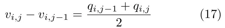
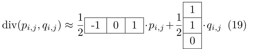
Now,plugging Eq.(17)into Eq.(14),the undefined quantities actually vanish,and one obtains:

In other words,the stencil for the Laplacian is replaced by

and that for the divergence by

The corresponding stencils for upper,left,and right borders are obtained by straightforward adaptations of this procedure.

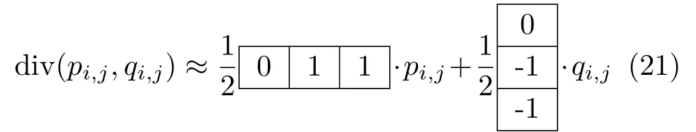
When two neighbours are missing.Boundary pixels having exactly two neighbours outsideΩare either“corners”(e.g.,(i,j−1)and(i+1,j)insideΩ,but(i−1,j)and(i,j+1)outsideΩ)or“lines”(e.g.,(i−1,j)and(i+1,j)insideΩ,but(i,j−1) and(i,j+1)outsideΩ).For“lines”,the natural boundary condition must be discretised four times (both forward and backward,on the two locations of missing data).Applying a similar rationale as in the previous case,we obtain the following stencils for“vertical”lines:

and

A straightforward adaptation provides the stencils for the“horizontal”lines.Applying the same procedure for corners,we obtain,for instance for the“top-left”corner:

and

Again,it is straightforward to find the other three discretisations for the other corner types.

When three neighbours are missing.In this last case,we discretise the boundary condition six times (forward and backward,for each missing neighbour). Most quantities actually vanish.For instance,for the case where only the right neighbour(i+1,j)is insideΩ,we obtain the following stencils:

and

In the end,we obtain explicit stencils for allfourteen types of boundary pixels.Let us emphasise that, apart from 4-connectivity,we make no assumption about the shape ofΩ.

Summarising the discretisation.The discretisation procedure defines a sparse linear system ofequationsAx=b.Incorporating Neumann boundary conditions,the matrixAis symmetric, positive semidefinite,diagonaldominant and its null space contains the vectore:=[1,...,1]T.In other words,Ais a rank-1 deficient,singular matrix.

2.3 Iterative Krylov subspace methods

As indicated,in consequence of enormous memory costs,application of a direct solver to deal with the above linear system appears to be impractical for large images.Therefore,we propose an iterative solver to handle this problem.

Krylov subspace solversare a modern class of iterative solvers designed for use with large sparse linear systems;for a detailed exposition see, e.g.,Refs.[31,41].The main idea behind the Krylov approach is to search for an approximate solution ofAx=b,whereA∈Rn×nis a large regular sparse matrix andb∈Rn,in a suitable low-dimensional(affine)subspace of Rnthat is constructed iteratively.

This construction is in general not directly visible in the formulation of a Krylov subspace method,as these are often described in terms of a reformulation whereAx=bis solved as an optimisation task. An important example is given by the classic conjugate gradient(CG)method of Hestenes and Stiefel[42]which is stillan adequate iterative solver for problems involving sparse symmetric matrices of the kind in Eq.(14)①While in general also positive definiteness is required,this point is more delicate.We comment later on the applicability in our case..

Conjugate gradient method.As it is ofspecial importance for this work,let us briefly recall some properties of the CG method;a more technical, complete exposition can be found in many textbooks on numerical computing(see,e.g.,Refs.[31,41,43, 44]).

Note that a useful implementation of CG is given in MATLAB.However,some knowledge of the technique is useful in order to understand some of its properties.Moreover,it is crucial for effective application of the CG method to be aware of its critical parameters.We now aim to make clear the relevant points.

The CG method requires a symmetric and positive definite matrixA∈Rn×n.In its construction it combines the gradient descent method with the method of conjugate directions.It can be derived from making use of the fact that,for such a matrix, the solution ofAx=bis exactly the minimum ofthe function:

since

here,〈·,·〉2means the Euclidean scalar product.

Let us now denote thekth Krylov subspace byKk. Then,Kk:=Kk(A,r0)is a subspace of Rndefined by

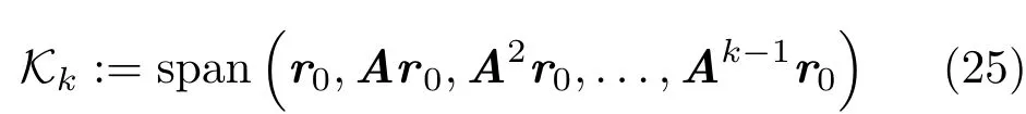
This meansKkis generated from an initial residual vectorr0=b−Ax0by successive multiplications by the system matrixA.

Let us briefly highlight some important theoretical considerations.The nature of an iterative Krylov subspace method is that the computed approximate solutionxkis inx0+Kk(A,r0),i.e.,it is determined by thekth Krylov subspace.Here,the indexkis also thekth iteration of the iterative scheme.

For the CG method,one can show that the approximate solutionsxkare optimal in the sense that they minimise the so-called energy norm of the error vector.Thus,ifx∗is a solution of the systemAx=b,thatxkminimises||x∗−xk||Afor theA-normNote again thatxkmust lie in thekth Krylov subspace.In other words, the CG method gives in thekth iteration the best solution available in the generated subspace.Since the dimension of the Krylov subspace increases in each step of the iteration,theoretical convergence is achieved at the latest after thenth step of the method if the solution is in Rn.

Practical issues.A usefulobservation on Krylov subspace methods is that they can obviously benefit from a good educated guess of the solution for use as the initial iteratex0.Therefore,we considerx0as an important open parameter of the method that should be addressed in a suitable way.

Moreover,an iterative method also requires the user to seta tolerance defining thestopping criterion: if the norm of the relative residual is below the tolerance,the algorithm stops.

However,there isa priorino means to say in which regime the tolerance has to be chosen.This is one of the issues that make reliable and efficient application of the method less than straightforward. It is one ofthe aims ofour experiments to determine a reasonable tolerance for our application.

While our presentation of the CG method relates to idealtheoreticalproperties,in practice,numerical rounding errors appear and very large systems may suffer from severe convergence problems. Thus,preconditioningis recommended to ensure all beneficial properties of the algorithm,along with fast convergence.However,as it turns out,it requires a thorough study to identify the most useful parameters in the preconditioning method.

Let us note that the CG method is applicable even though our matrixAis just positivesemidefinite. The positive definiteness is useful for avoiding division by zero within the CG algorithm.IfAis positive semidefinite,theoretically it may happen that one needs to restart the scheme using a different initialisation.In practice this situation rarely occurs.

Preconditioning.The basic idea of preconditioning is to multiply the original systemAx=bon the left by a matrixPsuch thatPapproximatesA−1.The modified systemPAx=Pbis in general better conditioned and much more efficient to solve.For sparseA,typical preconditioners are defined over the same sparse structure of entries ofA.

When dealing with symmetric matrices as in our case,incomplete Cholesky(IC)decomposition[45] is often used to construct a common and very efficient preconditioner for the CG method[46–48]. As a consequence of Ref.[29]we study here the application ofthe IC preconditioner and its modified version MIC.

Let us briefly describe the underlying ideas.The complete decomposition ofAis given byA=LLT+F.Ifthe lower triangular matrixLis allowed to have non-zero entries anywhere in the lower matrix,thenFis the zero matrix and the decomposition is the standard Cholesky decomposition.However,in the context ofsparse systems only the structure ofentries inAis used in definingL,so that the factorisation will be incomplete.Thus,in our case the lower triangular matrixLkeeps the same non-zero pattern as that ofthe lower triangular part ofA.The general form of the preconditioning then amounts to the transformation fromAx=btoApxp=bpwith

Practical issues.Let us identify another important computational parameter.The approach mentioned of taking the existing pattern inAas the sparsity pattern ofLis often called IC(0).If one extends the sparsity pattern ofLby additional non-zero elements(usually in the vicinity of existing entries)then the closeness between the productLLTandAmay be potentially improved.This procedure is often called a numerical fill-in strategy IC(τ), withdrop tolerance,where the parameterτ＞0 describes a dropping criterion[31We denote the combined methods of MIC(τ)and the shifted incomplete Cholesky version as MIC(τ,α).].The approach can be described as follows:new fill-ins are accepted only if the elements are greater than a local drop toleranceτ.It turns out that the corresponding PCG method is applicable for positive semidefinite matrices[49,50].

When dealing with a discretised elliptic PDE as in Eqs.(7)or(8),themodified IC(MIC)factorisation can lead to an even better preconditioner.For an overview of MIC see Refs.[43,48].The idea behind the modification is to force the preconditioner to have the same row sums as the original matrixA. This can be accomplished by adding dropped fill-ins to the diagonal.The latter is known as MIC(0)and can be combined with the drop tolerance strategy to MIC(τ).We note that MIC can lead to possible pivot breakdowns.This problem can be circumvented by a global diagonal shift applied toAprior to determining the incomplete factorisation[51]. Therefore,the factorisation①We denote the combined methods of MIC(τ)and the shifted incomplete Cholesky version as MIC(τ,α).of=A+αdiag(A) is performed,whereα＞0 and diag(A)is the diagonal part ofA.Note that the diagonal part ofAnever contains a zero value.

Adding fill-ins may obviously lead to a better preconditioner and a potentially better convergence rate.On the other hand,it becomes computationally more expensive to compute the preconditioner itself. Thus,there is a trade-off between speed and the improved convergence rate,an important issue upon which we will elaborate for our application.

2.4 On the FM-PCG normal integrator

Due to its localnature,the reconstructions computed by FM often have a lower quality compared to results of global approaches.On the other hand, the empowering effect ofpreconditioning the Poisson integration may still not suffice to achieve a high efficiency.The basic idea we follow now is that if one starts the PCG with a proper initialisationx0obtained by FM integration,instead of the standard casex0=0,the PCGnormalintegrator could benefit from a significant speed-up.This idea,together with dedicated numerical evaluation using a wellengineered choice of computational parameters for the numericalPCGsolver,is the core ofour proposed method.

In the following,we first given the important building blocks and parameters of our algorithm,in Section 3.It will become evident how theindividualmethods perform and how they compare.

After that we will show in Section 4 that our proposed FM-PCG normal integrator in whichsuitable building blocks are put togetheris highly competitive,and in many instances superior to the state-of-the-art methods for surface normal integration.

3 Numerical evaluation

We now demonstrate relevant properties of several state-of-the-art methods for surface normal integration.For this purpose,we give a careful evaluation regarding the accuracy of the reconstruction,the influence ofboundary conditions, flexibility to handle non-rectangular domains, robustness to noisy data,and computational efficiency—the main challenges for an advanced surface normal integrator.On the technical side,we note that the experiments were conducted on a i7 processor at 2.9 GHz.

Test datasets.To evaluate the proposed surface normal integrators,we provide examples of applications in gradient-domain image reconstruction(PET imaging,Poisson image editing)and surface-from-gradient(photometric stereo).Gradients of the“Phantom”and“Lena”images were constructed using finite differences, while both the surface and the gradient of the“Peaks”,“Sombrero”,and“Vase”datasets are analytically known,preventing any bias due to finite difference approximations.

We note that our test datasets demonstrate fundamental issues that one may typically find in gradient fields obtained from real-world problems: sharp gradients(“Phantom”),rapidly fluctuating gradients oriented in all grid directions in texturedareas(“Lena”),and smoothly varying gradient fields (“Peaks”).The gradient field of the“Vase”dataset has a non-trivial computational domain.

3.1 Existing integration methods

Fastandaccurate surface normal integrators are not abundant.For a meaningful assessment we compare our novel FM-PCG approach with the fast Fourier transform(FFT)method of Frankot and Chellappa[17]and the discrete cosine transform (DCT)extended by Simchony et al.[18]which are two of the most popular methods in use. Furthermore,we include the recent method of Harker and O’Leary[28]which relies on the formulation of the integration problem as a Sylvester equation.It is helpfulto consider in a first step the building blocks of our approach,i.e.,FM and CG-based Poisson integration separately.Hence,we also include in our comparison the FM method from Ref.[15].As for Poisson integration,only Jacobi[9,32]and Gauss–Seidel[27]iterations have been employed so far,so we consider Ref.[42]as a reference for CG-Poisson integration.

To highlight the differences between the methods, we start by comparing their algorithmic complexity, the type of admissible boundary conditions they admit,and the permissible the computational domainΩ:see Table 1.Algorithmic complexity is an indicator for the speed of a solver,while the admissible boundary conditions and the handling of non-rectangular domains influence its accuracy.The ability to handle non-rectangular domains improves also its computational efficiency.

The findings in Table 1 already indicate the potential usefulness of a mixture of FM and CG-Poisson approaches as both are free of constraints in the last two criteria and so their combination may lead to a reasonably computationally efficient Poisson solver.Although other methods have their strengths in algorithmic complexity and in the application of boundary conditions(apart from FFT),we see that the flexible handling of domains is a fundamental task and a key requirement of an ideal solver for surface normal integration.

Table 1 Comparison of five existing fast and accurate surface normal integration methods based on three criteria:their algorithmic complexity w.r.t.the numbernof pixels inside the computational domainΩ(the lower the better),the type of boundary condition (BC)they use(free boundaries are expected to reduce bias),and the permitted shape ofΩ(handling non-rectangular domains can be important for accuracy and algorithmic speed)

3.2 Stopping criterion for CG-Poisson

Amongst the considered methods,the Poisson solver (conjugate gradient method),where solving the discrete Poisson equation Eq.(7)corresponds to a linear systemAx=b,is the only iterative scheme. As indicated in Section 2.3,a practical solution can be reached quickly after a small numberkof iterations,butkcannot be predicted exactly.The general stopping criterion for an iterative method can be based on therelative residual(‖b−Ax‖)/‖b‖which we analyse in this paragraph.

To guarantee the efficiency of the CG-Poisson solver it is necessary to define the numberkof iterations depending on the quality of the reconstruction in the iterative process.To tackle this issue we compared the MSE③The mean squared error(MSE)is used to quantify the error of the reconstruction.We employed it to estimate the amount of the error contained in the reconstruction compared to the original.and the relative residual during each CG iteration.As the solution of the linear system Eq.(14)is not unique,an additive ambiguity+c,c∈R in the integration problem(cis the“integration constant”) occurs.Therefore,in each numerical experiment we chose the additive constantcwhich minimises the MSE,for fair comparison.To determine a proper relative residual,we considered the datasets“Lena”,“Peaks”,“Phantom”,“Sombrero”,and“Vase”on rectangular and non-rectangular domains.All test cases showed results similar to the graphs in Fig.1 for the reconstruction ofthe“Sombrero”surface(see Fig.2).

In this experiment the iterative solver CG-Poisson was stopped when the relative residual was lower than 10−6.However,it can be seen clearly that after around iteration 250,the quality measured by the MSE cannot be improved and therefore using more than 400 iterations is redundant.This numerical steady state ofthe MSE and therefore ofthe residual occurs when the relative residual is between 10−3and 10−4,so we use the suitable and“safe”stopping criterion of 10−4in subsequent experiments.

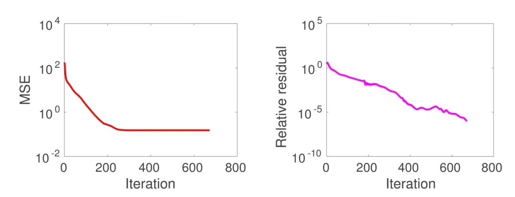
Fig.1 MSE vs.relative residual during CG iterations,for the“Sombrero”dataset.Although arbitrary relative accuracy can be reached,it is not useful to go beyond a 10−3residual,since such refinements have very small impact on the quality of the reconstruction,as shown by the MSE graph.Similar results were obtained for all datasets used in this paper.Hence,we set as stopping criterion a 10−4relative residual,which can be considered as“safe”.

Fig.2“Sombrero”surface(256×256)used in this experiment, whose gradient can be calculated analytically.Note that the depth values are periodic on the boundaries.

3.3 Accuracy of the solvers

First we analyse the general quality of the methods listed in Table 1 for the“Sombrero”dataset over a domain ofsize 256×256.In this example the gradient can be calculated analytically and furthermore the boundary conditions are periodic.Table 1 makes it obvious that all methods have no restrictions and consequently no discrimination.

Basically all methods provide a satisfactory reconstruction,and only FM produces a less accurate solution:see Figs.3 and 4.This can be seen more easily in Table 2,where the values of the measurements①We tested the two common measurements MSE and SSIM.A superior reconstruction has value closer to zero for MSE and a value closer to one for SSIM.The structural similarity(SSIM)index is a method for predicting the perceived quality of an image,see Ref. [52].of MSE and SSIM and the CPU time(in second)are given.The accuracy of all methods is similar,although the solution for FM,with 1.16 for MSE and 0.98 for SSIM,is slightly worse.In contrast the CPU time varies strongly,andin this case FFT and DCT,which need around 0.01 s, are unbeatable.The time for FM and Sylvester is in a reasonable range,and only the standard CGPoisson taking around 1.06 s being too slow and inefficient.For problems of surface reconstruction under these conditions,the choice ofa solver is fairly easy:the frequency domain methods FFT and DCT are best.

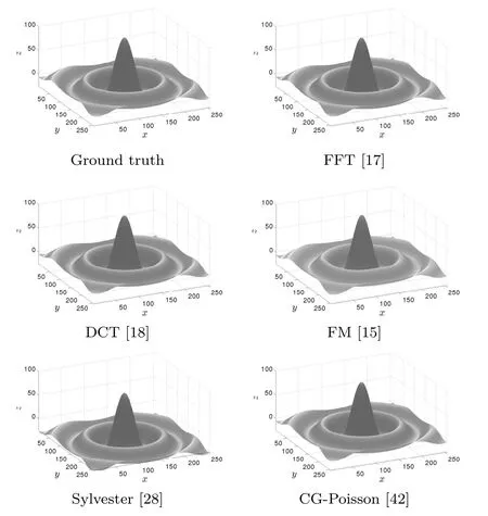
Fig.3 Results on the“Sombrero”dataset(cf.Table 2).

Fig.4 Absolute errors for the“Sombrero”dataset between the ground truth and the numerical result of each method;see Table 2. Note the diff erent scales of the plots.To highlight the diff erences between all methods we use three diff erent scales.The absolute error map of FM has its own scale due to the fact that the MSE and the maximum error diff er compared to the other methods.For FFT and DCT,Sylvester and CG respectively,which have similar values for the MSE and the maximum error,we used the same scale to point out the diff erences.

Table 2 Results on the“Sombrero”dataset(256×256). As expected,all methods provide reasonably accurate solutions. However,the FM result is slightly less accurate:this is due to error accumulation by thelocalnature of FM,while the other methods areglobal.The reconstructed surfaces are shown in Fig.3

3.4 Infl uence of boundary conditions

The handling of boundary conditions is a necessary issue which cannot be ignored.As we will show,different boundary conditions lead to surface reconstructions of different accuracy.The assumption of Dirichlet,periodic or homogeneous Neumann boundary conditions is often not justified and may even be unrealistic in some applications. A better choice is to use“natural”boundary conditions[2]of Neumann type.

The behaviour of the discussed solvers for unjustified boundary conditions,particularly for FFT,is illustrated by the“Peaks”dataset in Figs. 5 and 6 and the associated Table 3.Almost all methods provide good reconstructions;the FMresult is also acceptable.Only FFT,with 7.19 for MSE and 0.96 for SSIM,is strongly inferior and unusable for this real surface,as its accuracy is too low.

Our results show that FFT-based methods enforcing periodic boundary conditions can be discarded from the list of candidates for an idealsolver.Once again CG-Poisson is a very accurate integrator,but DCT and Sylvester are much faster and provide useful results.However,we may point out again in advance that enforcing the domainΩto be rectangular may lead to difficulties w.r.t. the transition from foreground to background of an object.

Table 3 Results on the“Peaks”dataset(128×128).Methods enforcing periodic BC fail to provide a good reconstruction.The reconstructed surfaces are shown in Fig.5

Fig.5 Results on the“Peaks”dataset(see Table 3).

3.5 Infl uence of noisy data

A key point in many applications is the question of the influence of noise on the quality of the reconstructions provided by different methods. Usually,the correctness of the given data,without noise,cannot be guaranteed.Therefore,it is essential to have a robust surface normal integrator with respect to noisy data.

To study the influence of noise,we should consider a dataset which,apart from noise,is perfect.Based on this aspect,a very reasonable test example is the“Sombrero”dataset;see Fig.2. The advantage of“Sombrero”is that the gradient of this object is known analytically,not just approximately.Furthermore,the computational domainΩis rectangular and the boundary conditions are periodic.For this test we added Gaussian noise with a standard deviationσvarying from 0%to 20%of‖[p,q]T‖∞to the known gradients①In the context of photometric stereo,it would be more realistic to add noise to the input images rather than to the gradients[53]. Nevertheless,evaluating the robustness of integrators given noisy gradients remains useful in order to compare their intrinsic properties..

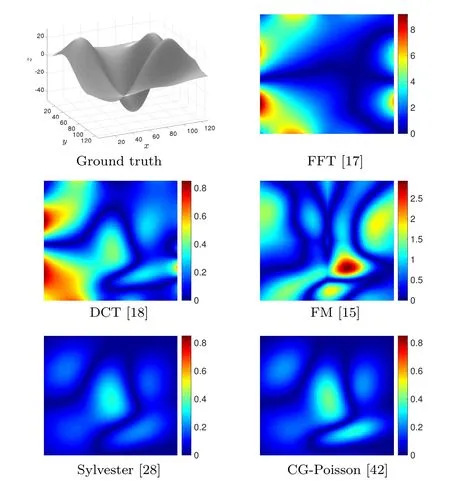
Fig.6 Absolute errors for the“Peaks”dataset between the ground truth and the numerical result of each method;see Table 3.Note the different scales of the plots.To highlight the differences between all methods we consider three diff erent scales.The absolute error maps of FFT and FM have their own scales due to the fact that the MSE and the maximum error are very diff erent in contrast to the other methods.For DCT,Sylvester,and CG,which have similar values for the MSE and the maximum error,we used the same scale to point out the diff erences.

The graph in Fig.7,which compares the MSE versus the standard deviation of Gaussian noise, indicates the robustness of the tested methods.The best performance is achieved by FFT,DCT,and CGPoisson,even for strong noisy data with a standard deviation of 20%.

The results of Sylvester are similar,but the method suffers from weaknesses in examples with noise of higher standard deviation,i.e.,larger than 10%.

As the FM integrator accumulates errors during front propagation,we observe,as expected,for highly noisy data this integrator is no longer a useful choice.

To conclude,if the accuracy of the given data is not known then FFT,DCT,and CG-Poisson are the safest integrators.

Fig.7 MSE as a function of the standard deviation of a Gaussian noise,expressed as percentage of the maximal amplitude of the gradient,added to the gradient.FFT,DCT,and CG-Poisson methods provide the best results for diff erent levels of Gaussian noise. The Sylvester method leads to reasonable results for a noise level lower than 10%.Since the FM approach propagates information in a single pass,it obviously also propagates errors,resulting in reduced robustness compared to all other approaches.

3.6 Handling non-rectangular domains

In this experiment we consider the situation when the gradient values are only known on a nonrectangular part of the grid.Applying methods needing rectangular grids[17,18,28]requires empirically fixing the values[p,q]:=[0,0]outsideΩ(see Fig.8),inducing a bias.

This can be explained as follows:filling the gradient with null values outsideΩcreates discontinuities between the foreground and background,preventing one from obtaining reasonable results,since all solvers considered here are intended to reconstruct smooth surfaces. This problem is illustrated in Figs.9 and 10 for the“Vase”dataset;Table 4 gives corresponding values for MSE and SSIM.

Fig.8 Mask for the“Vase”dataset.The gradient values are only known on a non-rectangular partΩof the grid,represented by the white region.The FM and the CG-Poisson integrators can handle easily any form of domainΩ.In contrast FFT,DCT,and Sylvester rely on a rectangular domain and therefore the values[p,q]:=[0,0] need to be fixed outsideΩ,in the black region.

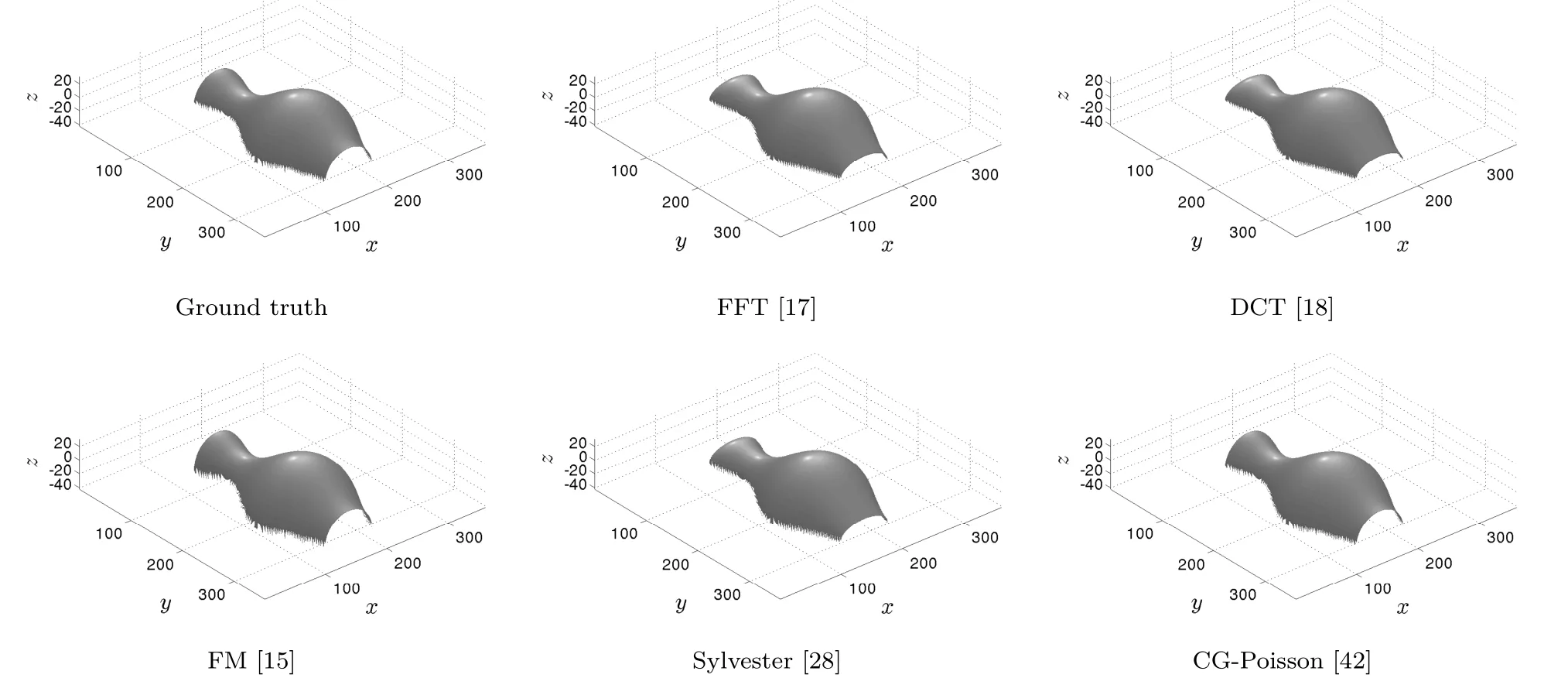
Fig.9 Results on the“Vase”dataset;see Table 4.

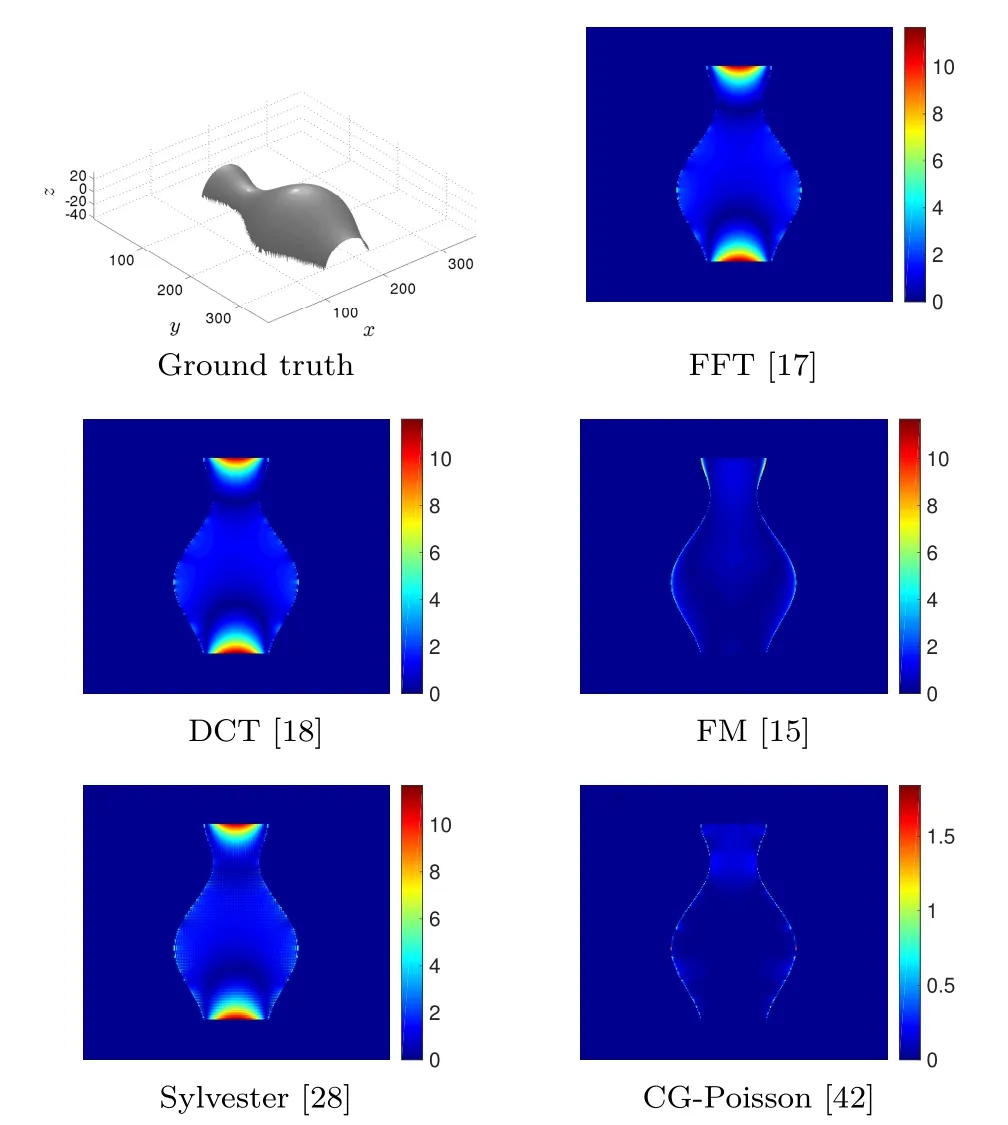
Fig.10 Absolute errors for the“Vase”dataset between the ground truth and the numerical result of each method;see Table 4.Note the diff erent scales of the plots.To highlight the diff erences between all methods we use two diff erent scales.The absolute error maps of FFT, DCT,Sylvester,and FM have the same scale due as their maximum errors are very close.For CG we use a diff erent scale to point out the diff erences.

The methods can be classified into two groups. In contrast to FM and CG-Poisson,FFT,DCT, and Sylvester methods,which cannot handle flexible domains,provide inaccurate reconstructions which are not useful.The non-applicability of these methods is a considerable problem,since realworld input images for 3D reconstruction are typically located within a photographed scene.This requires the flexibility to tackle non-rectangulardomains,while providing accurate(and efficient) reconstruction.

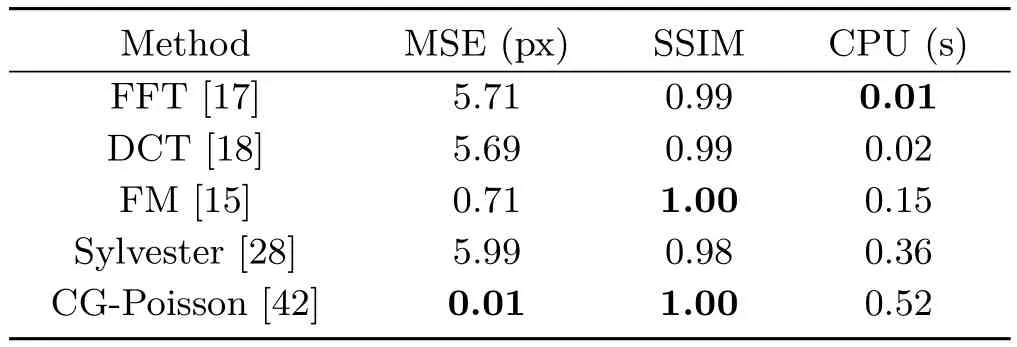
Table 4 Results on the“Vase”dataset(320×320).Methods dedicated to rectangular domains are clearly biased ifΩis not rectangular.The corresponding reconstructed surfaces are shown in Fig.9

This experiment shows that all methods except FM and CG-Poisson are not applicable as an ideal,high-quality normal integrator for many applications.

Let us note that we also have shown that FM and CG-Poisson have complementary properties and disadvantages:the former is fast but inaccurate, and the latter is slow but accurate.This clearly motivates the combination of FM as initialisation, and a Krylov-based Poisson solver:these should combine to give a fast and accurate solver.

3.7 Summary of the evaluation

In the previous experiments we tested different scenarios which arise in real-world applications.It was found that boundary conditions and noisy data may have a strong effect on 3D reconstruction.If rectangular domains can be considered,the DCT method seems to be a realistic choice of a normal integrator followed by Sylvester and CG-Poisson.In fact the first is unbeatably fast.However,the importance of handling non-rectangular domains, which is a practical issue in many industrial applications,cannot be underestimated.This situation leads to inaccuracies in the reconstructions of DCT and Sylvester methods.In this context FM and CG-Poisson methods achieve better results.

One can observe a certain lack of robustness w.r.t.noise of the FM integrator,especially along directions not aligned with the grid structure:see also the results in Ref.[29].This is because of the causality concept behind the FM scheme;errors that once appear are transported over the computational domain.This is not the case using Poisson reconstruction,which is a global approach and includes a regularising mechanism via the underlying least squares model.

Due to the possibly non-rectangular nature of the domains we aim to tackle,we cannot use fast Poisson solvers as,e.g.,in Ref.[18]to solve the discrete Poisson equations numerically.Instead,we explicitly construct linear systems and solve them using the CG solver as often done by practitioners. Nevertheless,the unmodified CG-Poisson solver is stillquite inefficient.

4 Accelerating CG-Poisson

Let us now demonstrate the advantages of the proposed FM-PCG approach compared to other state-of-the-art methods.In doing so,we give a carefulevaluation of allthe components ofour novel algorithm.

4.1 Preconditioned CG-Poisson

In a first step we analyse the behaviour of the CG solver when applying an additional preconditioner intended to improve the condition number and convergence speed w.r.t.the numberkof iterations, thus reducing time to reach the stopping criterion.

Fig.11“Phantom”image used in this experiment.Its gradient is unknown,so we approximate it numerically by first-order forward diff erences.We used this dataset for comparing preconditioners,for diff erent image sizes,from 64×64 to 4096×4096.

As examples of actual preconditioners,we examined①As pivot breakdowns for MIC(τ)are possible,we considered the shifted MIC version MIC(τ,α).All methods are predefined functions in MATLAB.IC(τ)and MIC(τ,α)for the test dataset“Phantom”(see Fig.11)for different input sizes. It was observed that MIC(τ,α∗)beats IC(τ)if we usedα∗=10−3for the global diagonal shift②This is an experimentally determined value..In the following,for simplicity we write MIC(τ)∗for MIC(τ,α∗)③If the valueτin MIC(τ)∗tends to zero then the preconditioned matrix is more dense,with more non-zero elements.As a consequence,the preconditioner is better;however it costs more time to compute the preconditioner itself..The results for MIC(0)∗,without a fill-in strategy,are shown in Table 5(third column) and demonstrate its usefulness compared to the nonpreconditioned CG-Poisson(second column).By using MIC(0)∗we save many iterations,greatly reducing the time taken:for example one can save around 2700 iterations and thus more than 1250 s for an image of size 4096×4096.

Now we show how useful a fill-in strategy can be. In columns four to eight we tested different fill-in strategies from MIC(10−1)∗to MIC(10−5)∗.A closer examination of Table 5 shows that MIC(10−3)∗provides the best balance between the time needed to compute the preconditioner and the time needed to apply PCG.As an example,again for the image of size 4096×4096,we can reduce the number of iterations from 247 to 80,taking around 170 s instead of 290 s.

Thus,the application of preconditioning,here shifted MIC,seems to be useful in accelerating the CG-Poisson integrator,but it is not sufficient to be competitive with common fast methods.However, we will see that with proper initialisation,this standard preconditioner can already be considered to be as efficient.

4.2 Appropriate initialisation

The suggested preconditioned CG-Poisson(PCGPoisson)method is not widely known in computer vision,although this practical method is surely not new and commonly used in numerical computing. However,we propose a novel scheme for the surface normalintegration(SNI)task,using an appropriateinitialisation to decrease the number of iterations and reduce the run time cost.Our proposed method consists of two steps:in a first step the FM solution is computed in a fast and efficient way;after that, the Krylov-based technique with shifted modified incomplete Cholesky(MIC)is applied.

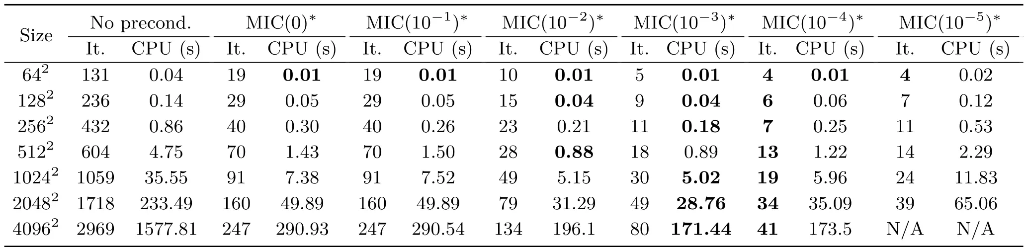
Table 5 Number of iterations and CPU time required to reach a 10−4relative residual for the conjugate gradient algorithm,using the shifted modified incomplete Cholesky(MIC)preconditioner(α∗=10−3)with diff erent drop tolerances and diff erent“Phantom”sizes.The 10−3drop tolerance is the one which provides the fastest results.Using a larger drop tolerance allows a reduced number of required iterations,but the time used for computing the preconditioner dramatically increases.Note that we were unable to compute the preconditioner MIC(10−5)∗for the 40962dataset,because 32 GB of memory was insufficient

To show the effect of the new FM initialisation, the test for the“Phantom”dataset was repeated and evaluated anew;see Table 6.Starting from the FM solution,which needs comparatively short computation time(see Table 7)even for large images, gives a dramatic speed-up.

A closer look at Tables 5 and 6 shows a significant difference,even without a fill-in strategy(compare both third columns).At first,let us consider the case without preconditioner:starting with the trivial solution leads to a constant increase in iterations (factor around 1.7)as the image size increases concomitantly.In contrast the number of iterations increases very slowly when using FM initialisation. The effect of this phenomenon is a notable,strong time cost reduction for large data:for 512×512 images,we can save more than 2 s(from 4.75 to 2.48 s),and for 4096×4096 images the time can be reduced from 1578 to 233 s.

Using additional preconditioning leads to similar results.Testing anew MIC(τ)∗with MIC(10−1)∗to MIC(10−5)∗shows once more that MIC(10−3)∗provides the best results;see Table 6.Using FM initialisation greatly reduces the required iterations to reach the stopping criterion and therefore the combination of FM and shifted MIC leads to fast reconstructions.In the case of an image of size 4096×4096,the novel approach,including the time taken to perform FMperforming of21.79 s(see Table 7),saves around 100 s(from 171 to 74 s)and 71 iterations compared with the trivialinitialisation and MIC(10−3)∗.

Finally,using the novel approach instead of the standard CG-Poisson solver leads to a significant speed-up;see Table 8.Without considering the computation of the FM initialisation,the construction of the system and the preconditioner, the time to purely solve the system is vastly reduced from 1552 to 19 s.The findings of this experiment show impressively that choosing FM asinitialisation accelerates the method greatly when it comes to standard preconditioners like(shifted modified)incomplete Cholesky.Thus,we believe that our novel FM-PCG method with shifted MIC preconditioning is a relevant contribution to the field of fast and accurate surface normal integrators.

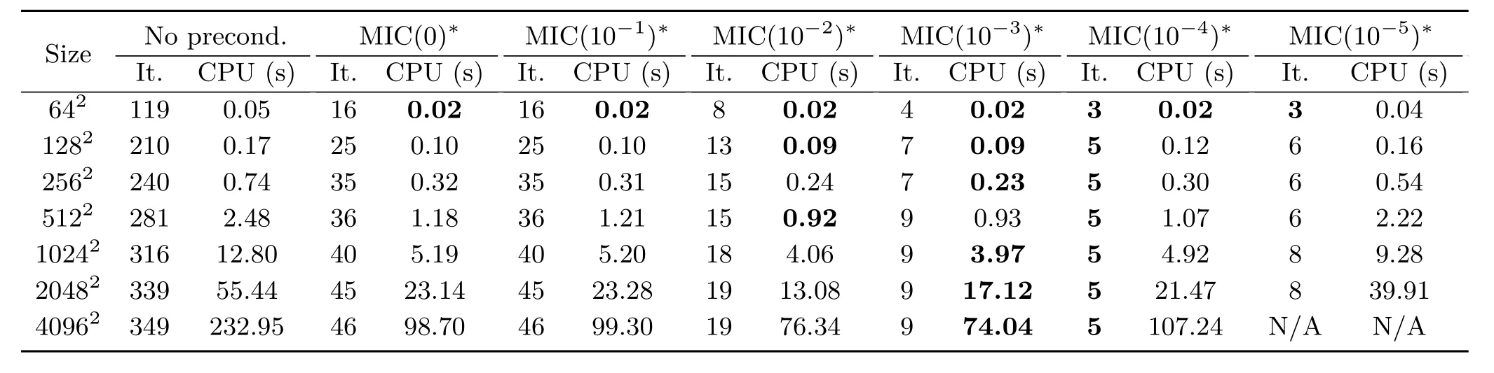
Table 6 Number of iterations and CPU time for applying the PCG algorithm,starting from the FM solution rather than from the trivial state.The indicated CPU time includes the time for computing the FM initialisation.Using FM as an initial guess saves many computations: the time to solve the 40962problem is reduced from 26 min(with neither FM initialisation nor preconditioning,see second column in Table 5, to 1 min(with FM initialisation and preconditioning,see column 6)

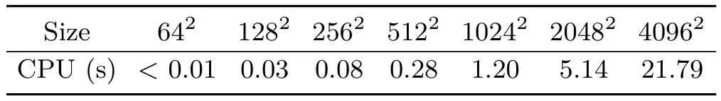
Table 7 CPU time to perform FM on the“Phantom”dataset of diff erent sizes

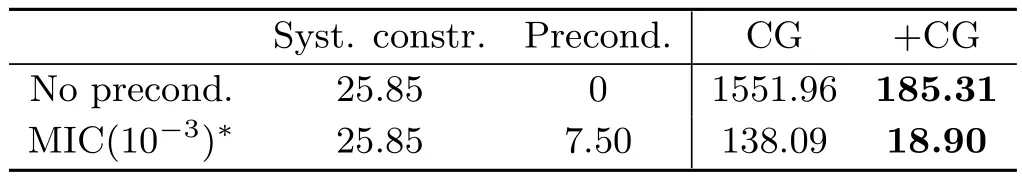
Table 8 Division of CPU time between system construction, preconditioning and system resolution,for the 40962example. Knowing that the system and the preconditioner can often be precomputed,this makes even more obvious the gain one can expect by choosing an appropriate initialisation such as the FM result.CG refers to the resolution of the system by conjugate gradient,and+CG to accelerated resolution by using FM initialisation(time does not include the 21.79 s required for FM)

4.3 Evaluation of the FM-PCG solver

To clarify the strength of our proposed FM-PCG solver against the standard FFT and DCT solvers and the“Sylvester”method of Harker and O’Leary, we use MSE to evaluate the reconstructions of the datasets“Phantom”,“Lena”,“Peaks”,and“Vase”on rectangular and non-rectangular domains. At first we examine the“Phantom”,“Lena”, and“Peaks”datasets on a rectangular domain in Tables 9–11.All examples contain the natural boundary equation;“Phantom”and“Lena”have sharp gradients and are more realistic.

It should be clear that FFT and DCT are the fastest methods,but the quality of FFT is inadequate and the results are unusable. Furthermore,it can be seen that the FM-PCG solver is the best integrator for sharp gradients(see Table 10).

Finally,the method with the best speed–quality balance on rectangular domains is probably DCT,followed by Sylvester and our proposed FM-PCG solver.However,as already mentioned,simple rectangular domains are quite unrealistic in many applications in science and industry.Hence,we analyse in Tables 12–15 the results on flexible domains,as shown in Fig.12.The given CPU time includes FM initialisation.

Table 9 Results on the“Phantom”dataset(1024×1024)

Table 10 Results on the“Lena”dataset(512×512)

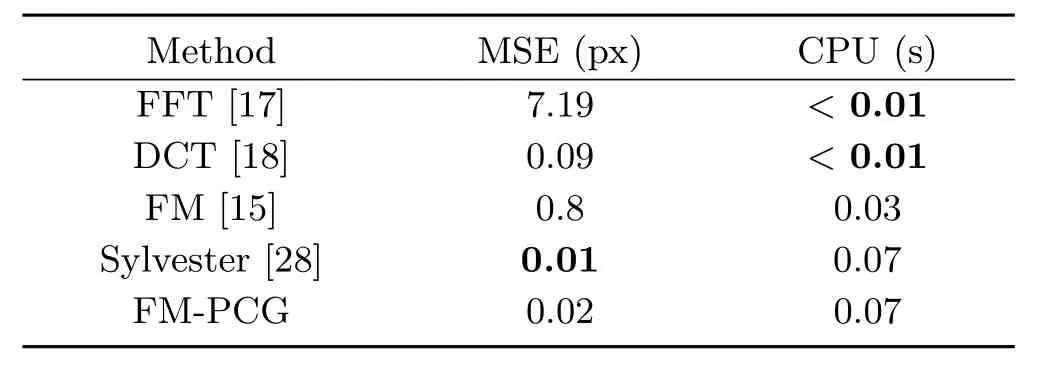
Table 11 Results on the“Peaks”dataset(128×128)

All experiments show the expected behaviour of the employed methods.The FM-PCG solution has by far the best quality.It is even faster than the Sylvester method.An assessment in relation to the best balance of speed versus quality is not easy and depends on the exact application.If speed is of secondary importance then the best choice is FMPCG,otherwise DCT.

4.4 Real-world photometric stereo data

The previous examples are rather simple.For this reason we consider a more realistic real-world application in photometric stereo,which definitely contains noisy data.We used the“Scholar”dataset①http://vision.seas.harvard.edu/qsfs/Data.html,which consists of 20 images of a Lambertian surface,taken from the same angle of view but under 20 known,non-coplanar lightings (see Fig.13).

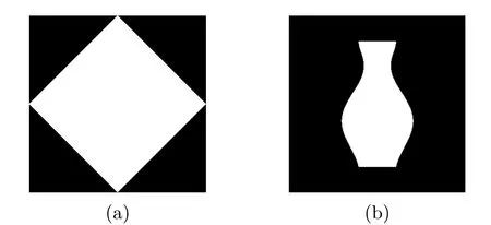
Fig.12 Masks for the“Phantom”,“Lena”,“Peaks”,and“Vase”datasets.It should be noted that FM and CG-Poisson work only on theΩrepresented by the white regions.By contrast,FFT, DCT,and Sylvester work on the whole rectangular domain.(a)The synthetic mask used for“Phantom”,“Lena”,and“Peaks”datasets. (b)Realistic mask for the“Vase”dataset.

Table 12 Results on the“Phantom”dataset for the non-rectangular domain in Fig.12(a)

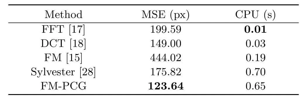
Table 13 Results on the“Lena”dataset for the non-rectangular domain in Fig.12(a)

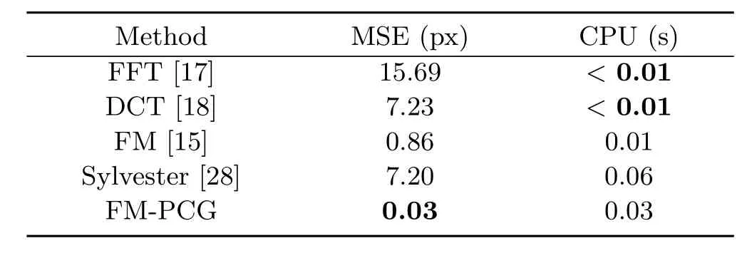
Table 14 Results on the“Peaks”dataset for the non-rectangular domain in Fig.12(a)

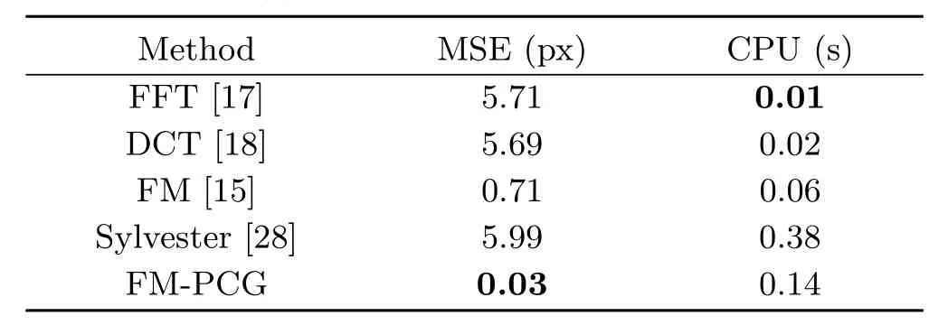
Table 15 Results on the“Vase”dataset for the non-rectangular domain in Fig.12(b)

The normals and the albedo were calculated using the classical photometric stereo approach of Woodham[3].Then,we integrated the normals using the diff erent solvers.Eventually,we a posteriori recomputed the normals by finite differences from the recovered depth map,before“reprojecting”the images using the estimated shape and albedo.By comparing the initial images with the reprojected ones,we obtain two criteria(MSE and SSIM) for evaluating the methods on each image.The results shown in Table 16 are the mean of the 20 corresponding values.

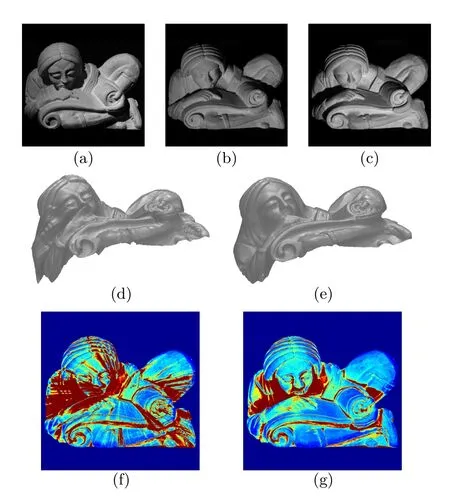
Fig.13 Application to photometric stereo(PS).(a)–(c)Three images(among 20),of size 1070×1070,acquired from the same point of view but under different lightings.After estimating the surface normals by PS,we integrated them by(d)FM,before(e)refining this initial guess by PCG iterations.The full integration process required a few seconds.(f)–(g)MSE(in pixel)of the reprojected images, computed from the surface estimated by(f)FM and(g)FM-PCG. (blue is 0,and red is＞1000).Due to the local nature of FM,radial propagation of errors is visible.After correction by CG,such artefacts are eliminated.Remaining bias is due to shadows.These results are experimentally compared with existing methods in Table 16.

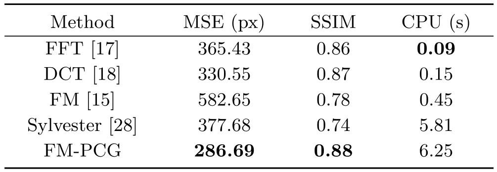
Table 16 Results on the PS dataset.Our method(initialisation by FM,then refinement by PCG from this initial guess)provides the most accurate results.We show the CPU time,as well as the mean MSE and SSIM for the 20 reprojected images

Once again FM-PCG is the most accurate integrator and is as fast as the Sylvester method. Nevertheless,the fast computational time of DCT was unbeatable.

4.5 Handling outliers

Let us now consider the case of standard photometric stereo applied to surfaces whose reflectance incorporates an additive non-Lambertiancomponent(specularities).As can be seen from Fig.14 and Table 17,all the integration methods we consider here are by their nature highly sensitive to outliers.

Fig.14(a)–(c)Three(out of 12)real-world images,of size 320×320,of a photometric stereo dataset.The eyes of the owl are highly specular.This induces a bias in the reconstructions,as shown in the reconstructions using(d)FMor(e)the proposed FM-PCG integrator. (f)–(g)The corresponding MSE of the reprojected images shows that the bias is very localized(blue is 0,and red is＞1000).

Table 17 Results on the specular PS dataset(see Fig.14).All methods present a similar systematic bias due to outliers located on the specular points

In order to handle such outliers,we replace the classic PI model in Eq.(7)by the modified model in Eq.(11).As already pointed out,all the methods relying on the Poisson equation can be adapted to this model.Therefore,we can employ here the FFT[17],DCT[18],and our new FMPCG methods.We found that using these modified inputs for the other SNI methods,such as FM[15] and Sylvester[28],also yields improved results. Hence,our improved model can be considered as agenericimprovement for use with existing SNI methods,enforcing robustness w.r.t.outliers.This is illustrated in Fig.15 and Table 18.

5 Conclusions and perspectives

We demonstrated the properties of the proposed FM-PCG surface normal integrator.It combines all the efficiency benefits of FM,Krylov-based and preconditioning components while retaining the robustness and accuracy of the underlying variational approach.

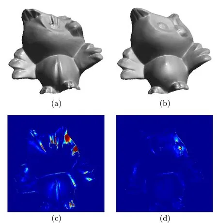
Fig.15 Results of(a)improved FM and(b)improved FM-PCG methods introducing a smoothness constraint on the outliers.The corresponding MSE maps(c)and(d)show that errors due to the outliers are much reduced.

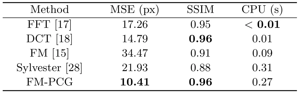
Table 18 Results of the improved methods on the same dataset as in Table 17.All MSE are significantly reduced

All of the desirable properties in Section 4, including especially the flexibility to handle nontrivial domains are met by the proposed method.It is clear that the proposed new integration scheme generates the most accurate reconstructions independently of the underlying conditions.The computational costs are very low and in most cases the method is faster than the recent Sylvester method of Harker and O’Leary.Only DCT is much faster,but DCT results are of low quality when the computational domain is not rectangular.

Therefore,the FM-PCGintegrator is a good choice for applications which require accurate and robust 3D reconstruction at relatively low computational cost.

Nonetheless,our integration method remains limited tosmoothsurfaces.Studying the impact of appropriate preconditioning and initialisation on iterative methods which allow depth discontinuities, as for instance Refs.[9,27],is an interesting problem.We are considering extending our study tomulti-viewnormal field integration[54]to be an exciting avenue,which would allow the recovery of a full 3D shape,instead of a depth map.

[1]P´erez,P.;Gangnet,M.;Blake,A.Poisson image editing.ACM Transactions on GraphicsVol.22,No. 3,313–318,2003.

[2]Horn,B.K.P.;Brooks,M.J.The variationalapproach to shape from shading.Computer Vision,Graphics and Image ProcessingVol.33,No.2,174–208,1986.

[3]Woodham,R.J.Photometric method for determining surface orientation from multiple images.Optical EngineeringVol.19,No.1,191139,1980.

[4]Zafeiriou,S.;Atkinson,G.A.;Hansen,M.F.;Smith, W.A.P.;Argyriou,V.;Petrou,M.;Smith,M. L.;Smith,L.N.Face recognition and verification using photometric stereo:The photoface database and a comprehensive evaluation.IEEE Transactions on Information Forensics and SecurityVol.8,No.1,121–135,2013.

[5]Smith,M.L.;Stamp,R.J.Automated inspection of textured ceramic tiles.Computers in IndustryVol.43, No.1,73–82,2000.

[6]Esteban,C.H.;Vogiatzis,G.;Cipolla,R.Multiview photometric stereo.IEEE Transactions on Pattern Analysis and Machine IntelligenceVol.30,No.3,548–554,2008.

[7]Haque,S.M.;Chatterjee,A.;Govindu,V.M. High quality photometric reconstruction using a depth camera.In:Proceedings of the IEEE Conference on Computer Vision and Pattern Recognition,2275–2282, 2014.

[8]Harker,M.;O’Leary,P.Least squares surface reconstruction from measured gradient fields.In: Proceedings of the IEEE Conference on Computer Vision and Pattern Recognition,1–7,2008.

[9]Durou,J.-D.;Aujol,J.-F.;Courteille,F.Integrating the normal field of a surface in the presence of discontinuities.In:Energy Minimization Methods in Computer Vision and Pattern Recognition.Cremers, D.;Boykov,Y.;Blake,A.;Schmidt,F.R.Eds. Springer Berlin Heidelberg,261–273,2009.

[10]Klette,R.;Schl¨uns,K.Height data from gradient fields.In:Proceedings of SPIE 2908,Machine Vision Applications,Architectures,and Systems Integration V,204–215,1996.

[11]Coleman Jr.,E.N.;Jain,R.Obtaining 3-dimensional shape of textured and specular surfaces using foursource photometry.Computer Graphics and Image ProcessingVol.18,No.4,309–328,1982.

[12]Wu,Z.;Li,L.A line-integration based method for depth recovery from surface normals.Computer Vision,Graphics and Image ProcessingVol.43,No. 1,53–66,1988.

[13]Robles-Kelly,A.;Hancock,E.R.A graphspectral method for surface height recovery.Pattern RecognitionVol.38,No.8,1167–1186,2005.

[14]Ho,J.;Lim,J.;Yang,M.H.;Kriegmann,D. Integrating surface normalvectors using fast marching method.In:Computer Vision–ECCV 2006.Leonardis, A.;Bischof,H.;Pinz,A.Eds.Springer Berlin Heidelberg,239–250,2006.

[15]Galliani,S.;Breuß,M.;Ju,Y.C.Fast and robust surface normal integration by a discrete eikonal equation.In:Proceedings of the 23rd British Machine Vision Conference,2012.

[16]B¨ahr,M.;Breuß,M.An improved eikonal method for surface normal integration.In:Pattern Recognition. Gall,J.;Gehler,P.;Leibe,B.Eds.Springer International Publishing,274–284,2015.

[17]Frankot,R.T.;Chellappa,R.A method for enforcing integrability in shape from shading algorithms.IEEE Transactions on Pattern Analysis and Machine IntelligenceVol.10,No.4,439–451,1988.

[18]Simchony,T.;Chellappa,R.;Shao,M.Direct analytical methods for solving Poisson equations in computer vision problems.IEEE Transactions on Pattern Analysis and Machine IntelligenceVol.12,No. 5,435–446,1990.

[19]Wei,T.;Klette,R.A wavelet-based algorithm for height from gradients.In:Robot Vision.Klette,R.; Peleg,S.;Sommer,G.Eds.Springer Berlin Heidelberg, 84–90,2001.

[20]Kovesi,P.Shapelets correlated with surface normals produce surfaces.In:Proceedings of the 10th IEEE International Conference on Computer Vision,Vol.2, 994–1001,2005.

[21]Wei,T.;Klette,R.Depth recovery from noisy gradient vector fields using regularization.In:Computer Analysis of Images and Patterns.Petkov,N.; Westenberg,M.A.Eds.Springer Berlin Heidelberg, 116–123,2003.

[22]Kara¸cali,B.;Snyder,W.Noise reduction in surface reconstruction from a given gradient field.International Journal on Computer VisionVol.60,No. 1,25–44,2004.

[23]Agrawal,A.;Raskar,R.;Chellappa,R.What is the range of surface reconstructions from a gradient field? In:Computer Vision–ECCV 2006.Leonardis,A.; Bischof,H.;Pinz,A.Eds.Springer Berlin Heidelberg, 578–591,2006.

[24]Badri,H.;Yahia,H.M.;Aboutajdine,D. Robust surface reconstruction via triple sparsity.In: Proceedings of the IEEE Conference on Computer Vision and Pattern Recognition,2283–2290,2014.

[25]Du,Z.;Robles-Kelly,A.;Lu,F.Robust surface reconstruction from gradient field using the L1 norm. In:Proceedings of the 9th Biennial Conference of the Australian Pattern Recognition Society on Digital Image Computing Techniques and Applications,203–209,2007.

[26]Reddy,D.;Agrawal,A.K.;Chellappa,R.Enforcing integrability by error correction usingl1-minimization. In:Proceedings of the IEEE Conference on Computer Vision and Pattern Recognition,2350–2357,2009.

[27]Qu´eau,Y.;Durou,J.-D.Edge-preserving integration of a normal field:Weighted least squares,TV and L1approaches.In:Scale Space and Variational Methods in Computer Vision.Aujol,J.-F.;Nikolova,M.; Papadakis,N.Eds.Springer International Publishing 576–588,2015.

[28]Harker,M.;O’Leary,P.Regularized reconstruction of a surface from its measured gradient field.Journal of Mathematical Imaging and VisionVol.51,No.1,46–70,2015.

[29]Breuß,M.;Qu´eau,Y.;B¨ahr,M.;Durou,J.-D.Highly efficient surface normal integration.In:Proceedings of the 20th Conference on Scientific Computing,204–213, 2016.

[30]Meister,A.Comparison of diff erent Krylov subspace methods embedded in an implicit finite volume scheme for the computation of viscous and inviscid flow fields on unstructured grids.Journal of Computational PhysicsVol.140,No.2,311–345,1998.

[31]Saad,Y.Iterative Methods for Sparse Linear Systems. Society for Industrialand Applied Mathematics,2003.

[32]Durou,J.-D.;Courteille,F.Integration of a normal field without boundary condition.In:Proceedings of the 1st International Workshop on Photometric Analysis for Computer Vision,2007.

[33]Kimmel,R.;Sethian,J.A.Optimal algorithm for shape from shading and path planning.Journal of Mathematical Imaging and VisionVol.14,No.3,237–244,2001.

[34]Tsitsiklis,J.N.Efficient algorithms for globally optimaltrajectories.IEEE Transactions on Automatic ControlVol.40,No.9,1528–1538,1995.

[35]Sethian,J.A.A fast marching level set method for monotonically advancing fronts.Proceedings of the National Academy of Sciences of the United States of AmericaVol.93,No.4,1591–1595,1996.

[36]Helmsen,J.J.;Puckett,E.G.;Colella,P.;Dorr, M.Two new methods for simulating photolithography development in 3D.In:Proceedings of SPIE 2726, Optical Microlithography IX,253–261,1996.

[37]Sethian,J.A.Level Set Methods and Fast Marching Methods:Evolving Interfaces in Computational Geometry,Fluid Mechanics,Computer Vision,and Materials Science.Cambridge University Press,1999.

[38]Yatziv,L.;Bartesaghi,A.;Sapiro,G.O(N) implementation of the fast marching algorithm.Journal of Computational PhysicsVol.212,No.2, 393–399,2006.

[39]Cacace,S.;Cristiani,E.;Falcone,M.Can local single-pass methods solve any stationary Hamilton–Jacobi–Bellman equation?SIAM Journal on Scientific ComputingVol.36,No.2,A570–A587,2014.

[40]Zimmer,H.;Bruhn,A.;Valgaerts,L.;Breuß,M.; Weickert,J.;Rosenhahn,B.;Seidel,H.-P.PDE-based anisotropic disparity-driven stereo vision.In: Proceddings of the 13th International Fall Workshop Vision,Modeling,and Visualization,263–272,2008.

[41]Meister,A.Numerik Linearer Gleichungssysteme. Eine Einf¨uhrung in Moderne Verfahren.Springer Spektrum,2014.

[42]Hestenes,M.R.;Stiefel,E.Methods of conjugate gradients for solving linear systems.Journal of Research of the National Bureau of StandardsVol.6, No.49,46–70,1952.

[43]Meurant,G.Computer Solution of Large Linear Systems.Elsevier Science,1999.

[44]Meurant,G.The Lanczos and Conjugate Gradient Algorithms:From Theory to Finite Precision Computations.Society for Industrial and Applied Mathematics,2006.

[45]Golub,G.H.;van Loan,C.F.Matrix Computation, 3rd edn.Johns Hopkins,1996.

[46]Meijerink,J.A.;van der Vorst,H.A.An iterative solution method for linear systems of which the coefficient matrix is a symmetricM-matrix.Mathematics of ComputationVol.31,No.137,148–162,1977.

[47]Kershaw,D.S.The incomplete Cholesky-conjugate gradient method for the iterative solution of systems of linear equations.Journal of Computational PhysicsVol.26,No.1,43–65,1978.

[48]Benzi,M.Preconditioning techniques for large linear systems:A survey.Journal of Computational PhysicsVol.182,No.2,418–477,2002.

[49]Kaasschieter,E.F.Preconditioned conjugate gradients for solving singular systems.Journal of Computational and Applied MathematicsVol.24,Nos. 1–2,265–275,1988.

[50]Tang,J.M.;Vuik,C.Acceleration of preconditioned Krylov solvers for bubbly flow problems.In:Parallel Processing and Applied Mathematics.Wyrzykowski, R.;Dongarra,J.;Karczewski,K.;Wasniewski,J.Eds. Springer Berlin Heidelberg,1323–1332,2008.

[51]Manteuff el,T.A.An incomplete factorization technique for positive definite linear systems.Mathematics of ComputationVol.34,No.150, 473–497,1980.

[52]Wang,Z.;Bovik,A.C.;Sheikh,H.R.;Simoncelli, E.P.Image quality assessment:From error visibility to structural similarity.IEEE Transactions on Image ProcessingVol.13,No.4,600–612,2004.

[53]Noakes,L.;Kozera,R.Nonlinearities and noise reduction in 3-source photometric stereo.Journal of Mathematical Imaging and VisionVol.18,No.2,119–127,2003.

[54]Chang,J.Y.;Lee,K.M.;Lee,S.U.Multiview normal field integration using level set methods.In: Proceedings of the IEEE Conference on Computer Vision and Pattern Recognition,1–8,2007.

Martin B¨ahr is a Ph.D.student in mathematics at the Brandenburg Technical University in Germany.He received his master degree in applied mathematics at the same university in 2013.Since 2013,he works in the applied mathematics group with a scientific focus on mathematical image processing.His research interests include partialdiff erential equations and numerical methods for image processing and computer vision.

Yvain Qu´eau is a postdoctoral researcher at Technical University Munich.He received his Ph.D. degree in computer science from INPENSEEIHT,Universit´e de Toulouse, in 2015.His research interests include 3D-reconstruction by photometric techniques(shape-from-shading and photometric stereo),as well as variational methods for solving computer vision and image processing problems.

Ali SharifiBoroujerdi is a Ph.D. student at the Brandenburg Technical University in Germany.After being a bachelor of software engineering,he received his master degree in software engineering in 2013.His research interests include dynamic programming techniques as well as the field of artificial intelligence in general,especially deep learning, reinforcement learning,and big data analysis.

Jean-Denis Durou received his Ph.D.degree in computer science from the Universit´e Paris Sud-Orsay in 1993,and the“Habilitation`a Diriger les Recherches”from the Universit´e Toulouse III-Paul Sabatier in 2007. He is an assistant professor at the Universit´e Toulouse III since 1994,and a member of the VORTEX team at the IRIT Laboratory. His main research interest is 3D-vision.He is more specifically interested in photometric 3D-reconstruction, i.e.,shape-from-shading and photometric stereo.

Open Access The articles published in this journal are distributed under the terms of the Creative Commons Attribution 4.0 International License(http:// creativecommons.org/licenses/by/4.0/),which permits unrestricted use,distribution,and reproduction in any medium,provided you give appropriate credit to the original author(s)and the source,provide a link to the Creative Commons license,and indicate if changes were made.

Other papers from this open access journalare available free of charge from http://www.springer.com/journal/41095. To submit a manuscript,please go to https://www. editorialmanager.com/cvmj.

reuß

his doctorate degree in mathematics from the University of Hamburg in 2001,and the habilitation in mathematics from the Technical University in Brunswick in 2006.For several years,he had been a member of the mathematical image analysis group in Saarbr¨ucken, Germany.Since 2016,he is professor for applied mathematics at the Brandenburg Technical University in Cottbus,Germany.His research interests are mainly in mathematical image processing and 3D vision,and include in particular numerical methods.

1 Brandenburg Technical University,Institute for Mathematics,Chair for Applied Mathematics,Platz der Deutschen Einheit 1,03046 Cottbus,Germany. E-mail:M.B¨ahr,martin.baehr@b-tu.de;M.Breuß, michael.breuss@b-tu.deA.S.Boroujerdi,ali. sharifiboroujerdi@b-tu.de.

2 Technical University Munich,85748 Garching,Germany. E-mail:yvain.queau@tum.de.

3 Universit´e de Toulouse,IRIT,UMR CNRS 5505, Toulouse,France.E-mail:durou@irit.fr.

Manuscript received:2016-10-18;accepted:2016-12-21