A new three-dimensional finite-volume non-hydrostatic shock-capturing model for free surface flow*

Francesco Gallerano, Giovanni Cannata, Francesco Lasaponara, Chiara Petrelli

Department of Civil, Constructional and Environmental Engineering, Sapienza University of Rome, Rome, Italy, E-mail:francesco.gallerano@uniroma1.it

A new three-dimensional finite-volume non-hydrostatic shock-capturing model for free surface flow*

Francesco Gallerano, Giovanni Cannata, Francesco Lasaponara, Chiara Petrelli

Department of Civil, Constructional and Environmental Engineering, Sapienza University of Rome, Rome, Italy, E-mail:francesco.gallerano@uniroma1.it

In this paper a new finite-volume non-hydrostatic and shock-capturing three-dimensional model for the simulation of wave-structure interaction and hydrodynamic phenomena (wave refraction, diffraction, shoaling and breaking) is proposed. The model is based on an integral formulation of the Navier-Stokes equations which are solved on a time dependent coordinate system: a coordinate transformation maps the varying coordinates in the physical domain to a uniform transformed space. The equations of motion are discretized by means of a finite-volume shock-capturing numerical procedure based on high order WENO reconstructions. The solution procedure for the equations of motion uses a third order accurate Runge-Kutta (SSPRK) fractional-step method and applies a pressure corrector formulation in order to obtain a divergence-free velocity field at each stage. The proposed model is validated against several benchmark test cases.

Three-dimensional simulation,non-hydrostatic,wave-structure interaction,flow-structure interaction,shock-capturing

Introduction

Since 1960s several studies have been conducted to evaluate hydrodynamic phenomena related to wave motion. Since computational capabilities were exiguous, just a few models have been developed to make these simulations. As the computational power advanced a few new approaches of modelling surface waves have been developed and became more popular. One was based on the depth-averaged equations, such as shallow water equation models[1-3]or Boussinesq equation models[4,5]. The depth-averaged models are computationally efficient with the trade-off of losing depthrelated information.

The most recent Boussinesq models have very good dispersion and nonlinearity properties[6-11]and some models even retain the second order vertical vorticity component[12,13]. These models so-called“depth averaged” are still very popular in coastal engineering for example to study coastal flooding dueto tsunami[14,15]or in sediment transport field[16]. These models are even used in all coastal simulation for which the vertical distribution of hydrodynamic quantities is not necessary. However, in order to solve three-dimensional engineering problems, models that take into account the three-dimensionality of the vorticity and turbulent phenomena are required. A different approach, commonly used in the past, is to solve the Navier-Stokes equations by the assumption of hydrostatic pressure. The pioneers in these studies were Johns and Jefferson[17]and Casulli and Cheng[18]. Due to the employment of the hydrostatic pressure assumption, such models are generally applied to shallow water flows. When the vertical acceleration of fluids is strong,i.e.,wave impacton structures, the models may fail to provide accurate results[19].

In several applications, the vertical acceleration might not be negligible compared to the gravity acceleration, mostly to simulate highly dispersive and nonlinear phenomena in deep and intermediate water. For these reasons the most recent models take into account the dynamic pressure[20-25]. The “free surface fully non-hydrostatic three-dimensional models” did not become popular before the XXI century, when the computational power greatly increased. In these models the total pressure is split into two parts: the dyna-mic pressure and the hydrostatic pressure. The governing equations are solved in two different steps: in the first step the convective terms, the hydrostatic pressure, the term related to the bottom slope and the stress term are discretized. In the second step the dynamic pressure is calculated by solving the so-called Poisson equation. The first “free surface fully non-hydrostatic models” were solved by using Cartesian coordinates[26-28],by this way vertical fluxes cross the calculus cell arbitrarily. This led to the difficulty of correctly assigning the free surface elevation pressure kinematic condition. Also, Cartesian coordinates are not able to represent complex bottom topography. This approach led to the presence of spurious oscillations in the numerical solution and requested an high number of vertical layers[23]. A direct simplification of the above-mentioned approach is to express the vertical coordinate as a function of quantities that depends only by horizontal coordinates. By this way the physical grid (Cartesian grid) is mapped to a computational grid (sigma-coordinate[29]) which has always a rectangular prism shape. By doing so, the free surface is always located at the upper computational boundary and the bottom is always located at the lower computational boundary and they can be determined by applying the free surface and bottom boundary conditions. Furthermore, the pressure boundary condition at the free surface can be exactly assigned to zero without any approximation[[2233]]. The integral form of the motion equations, expressed in terms of conserved variables, guarantees that high-order shock-capturing numerical schemes converge to correct weak solutions and are then able to directly simulate the wave breaking and the energy dissipation associated with it[30]. These schemes are shock-capturing methods and are able to track the actual location of the wave breaking without requiring any criterion[21].

In this paper, the numerical simulation of wave transformation relies on the resolution of the governing equations expressed in an integral formulation on a time dependent coordinate system: a coordinate transformation maps the varying coordinates in the physical domain to a uniform transformed space. The pressure boundary conditions are placed on the upper face of each computational cell. The solution procedure for motion equations uses a third order accurate Runge-Kutta (SSPRK) fractional-step method and applies a pressure corrector formulation in order to obtain a divergence free velocity field at each stage. In the prediction phase of the fractional-step proposed model, the motion equations are discretized by means of a shock-capturing numerical procedure based on high order WENO reconstructions[31]. The numerical flux is given at each cell interface by the solution of an approximate HLL Riemann problem[32]. In the corrector phase of the fractional-step proposed model, in order to solve the Poisson equation and reduce the computational costs related to it, an alternate fourcolour Zebra line Gauss-Seidel relaxation method with a V-cycle multigrid strategy is used[33]. In order to further reduce computational costs, the proposed model has been fully parallelized with message passing interface (MPI).

1. An integral form of three-dimensional sigmacoordinate equations

The integral form of the momentum equations over a control volumeΔV( t)which varies in time is given by

where ΔA( t)is the surface of the control volume, nm(m=1,3)is the outward unit normal vector to the surface ΔA( t), ul( l=1,3)and vm(m=1,3)are respectively the fluid velocity and the velocity of the surface of the control volume, both defined in a Cartesian reference system of coordinates xl(l=1,3), ρis the density of the fluid, Tlmis the stress tensor and fl(l=1,3)represents the external body forces per unit mass vector

in which δ13is the Kroneker symbol and pis the total pressure defined by the sum of the hydrostatic and the dynamic component

where Gis the constant of gravity, qis the dynamic pressure, ηis the free surface elevation, the comma with an index in subscript denotes the derivative asandis a Cartesian coordinate system. The first integral on the right hand side of Eq.(1)can be rewritten as

By applying Green’s theorem the right hand side of Eq.(4)becomes

By introducing Eq.(5)in Eq.(1), we get

In order to simulate the fully dispersive wave processes, Eq.(6)can be transformed in the following way. Letwhere his the depth of still water. Our goal is to accurately represent the bottom and surface geometry and correctly assign pressure and kinematics conditions on bottom and free surface elevation. Let (ξ1, ξ2,ξ3,τ) be a system of curvilinear coordinates which varies in time so as to follow the time variation of the free surface elevation,the transformation from the Cartesian coordinates (x1, x2,x3, t)to the curvilinear coordinates (ξ1, ξ2,ξ3,τ)is

The following relation is valid

This coordinate transformation basically maps the varying vertical coordinates in the physical domain to a uniform transformed space where3ξ spans from 0 to 1.

For an incompressible fluid, Eq.(6), in which the external body forces are given by the only gravitational force, becomes

The time dependent coordinate system moves with velocity given by. The first integral on the right hand side of Eq.(9)is related to the convective term and the hydrostatic pressure gradient, the second integral on the right hand side is related to the dynamic pressure gradient and the third term is related to the stress tensor.

We define the transformation matrixand its inverseThe metric tensor and its inverse are defined byand, respectively. The Jacobian of the transformation is defined byIt is not difficult to verify that in the particular case of the above-mentioned transformation

Let us introduce a restrictive condition on the volume element ΔV( t): in the following ΔV( t) must be considered as a volume element defined by surface elements bounded by curves lying on the coordinate lines. Consequently, we define the volume elementin the physical space, and the volume element in the transformed spaceIt is possible to see that the first volume element is time dependent while the second one is not. In the same way we define the surface element in the physical spaceand the surface element in the transformed space ΔA*=ΔξαΔξβ(in which α, β=1,2,3are cyclic). We define the averaged cell value (in the transformed space) of primitive variables

and conserved variable

By using Eqs.(10)-(11), the expression of Eq.(9)in the time dependent coordinate system(ξ1, ξ2,ξ3,τ) (transformed from the Cartesian reference system of coordinates (x1, x2,x3, t)by Eq.(7)), in which the velocity vectorsuland vmare defined in the Cartesian reference system, is transformed in

where ΔA*α+and ΔA*α-indicate the contour surfaces of the volume element ΔV*on which ξαis constant and which are located at the larger and at the smaller value ofαξrespectively. Here the indexes α, βand γare cyclic. The total time derivative on the left hand side of Eq.(9)has become a local time derivative (Eq.(12)) because the integral is a simple function of (ξ1, ξ2,ξ3,τ). It is possible to see that the advancing in time of the conserved variables is applied in the transformed space that is not time varying. The time varying of the geometric components is expressed by the metric terms.

The mass conservation principle is given by

The integral form of the continuity equation expressed in a time dependent coordinate system is given by

By treating ρas a constant and uniform value, Eq.(14)becomes

By developing the summation, Eg.(15) reads

Because Hdoes not depend on ξ3and ΔV*is not time dependent. We can also write

By considering the bottom and surface kinematic boundary conditions, by using Eq.(10), Eqs.(17)-(18) and by dividing Eq.(16)by, we obtain

in which ξα+and ξα-indicate the contour lines of the surface element ΔA*on which ξαis constant and which are located at the larger and at the smaller value ofrespectively. Equation (19)represents the governing equation for the surface movements. Eq.(12)and Eq.(19)represent the expressions of the three-dimensional motion equations as a function of theand Hvariables in the time dependent coordinate system (ξ1, ξ2,ξ3,τ). The numerical integration of the above mentioned Eq.(12)and Eq.(19) allows the fully dispersive wave processes simulation.

The turbulent kinematic viscosity in the stress tensor is estimated by a Smagorinsky sub grid model.

2. Numerical scheme

A combined finite-volume and finite-difference scheme with a Godunov-type method has been applied in order to discretize Eq.(12)and Eq.(19). By following the strategy described by Stelling and Zijlema[34]a particular kind of staggered grid framework is introduced, in which the velocities are placed at the cell centers and the pressure is defined at the horizontal cell faces. The state of the system is known at the centre of the calculation cells and it is defined by the cell-averaged values Huland H. τ(n)is the time level of the known variables while τ(n+1)is the time level of the unknown variables. The solution procedure uses a three-stage third-order nonlinear strong stability-preserving (SSP) Runge-Kutta scheme[35]for Eq.(12)and Eq.(19). A pressure correction formulation is applied in order to obtain a divergence free velocity field at each time level. Withknown,is calculated with the following three stage iteration procedure.

Let

At each stage p(where p=1,2,3) an auxiliary fieldare obtained directly from* Eq.(12)by using values from the previous stage

Equation(22), expressed in the time dependent coordinate system, is given by

The corrector irrotational velocity field is calculated by the following expressions:

in order to obtain a divergence-free velocity field at each stage and a non-hydrostatic velocity field, the velocity field must be corrected as

For the calculation of the D( H, ul,τ)and L( H, ul,τ)terms the numerical approximations of the integrals on the right hand side of Eq.(12)and Eq.(19)is required.

The aforementioned calculation is based on the following sequence.

(1)High order WENO reconstructions, from cell averaged values, of the point values of the unknown variables at the centre of the contour faces which define the calculation cells. At the centre of the contour face which is common with two adjacent cells, two point values of the unknown variables are reconstructed by means of two WENO reconstruction defined on two adjacent cells[11].

(2)Advancing in time of the point values of the unknown variables at the centre of the contour faces by means of the so-called solution of the HLL Riemann problem[32], with initial data given by the pair of point-values computed by two WENO reconstructions defined on the two adjacent cells.

(3)Calculation of the spatial integrals which define D( H, ul,τ)and L( H, ul,τ).

(4)Solution of the Poisson pressure equation by using a four-colour Zebra line Gauss-Seidel alternate method and a multigrid V-cycle.

(5)Correction of the hydrostatic velocity field by using a scalar potential Ψ.

(6)Advancing in time of the total local depth (Eq.(19)) by using the non-hydrostatic velocity field.

3. Results

3.1 Standing wave in closed basin

For a hydrodynamic non-hydrostatic model, the ability to preserve the wave shape is a basic requirement. In the case of a three-dimensional hydrodynamic non-hydrostatic model, the model’s dispersion properties depend on the horizontal and vertical spatial discretization. It is therefore possible to improve the three-dimensional model dispersion properties by increasing the number of vertical layers. Because of the computational costs which can result from this increase, a good three-dimensional model should at the same time guarantee good dispersion properties and few vertical layers.

In this section the dispersion properties of the proposed hydrodynamic model are verified by reproducing a test case proposed by Casulli and Stelling[28]and used by several authors[34,38,23]. This test consists in the simulation of a standing wave in a closed basin with lengthL=20 mand depth H=10 m. Starting with zero initial velocity, the flow is driven by an initial free surface elevation given by η=acos(kx) where a=0.1mis the amplitude of the standing wave and k=π/His the wave number for this test case. Since kH=πis significantly greater than one, this wave is highly dispersive. The expected solution (calculated by applying the Airy wave theory) consists of a standing wave of length equal to the length of the basin and period T=3.59 s . The numerical test is made by using a time step of 0.002 s and a finely resolved horizontal grid obtained by discretising the horizontal length of the basin by 102 calculation cells. In order to test the proposed model dispersion properties as a function of the number of vertical layers, the depth of the basin is discretized by adopting the same numbers of vertical layers (3, 5, 8, 10) used by Ma et al.[23]. The simulation time is 30 s. The comparison between numerical results is show in Fig.1.

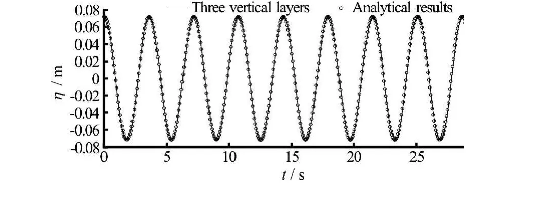
Fig.1 Standing wave in closed basin.Comparison between numerical results of the surface elevation at x=17.5m

In Fig.2 the curve indicated with the continuous line (proposed model) shows how the numerical errordecreases as the number of vertical layers increases. The numerical errors are calculated by using the expression proposed by Ma et al.[23]

in which Ais the wave amplitude, Nis the number of data that are compared,iηis the value obtained by the numerical simulation andαηis the value of the analytical solution.

Fig.2 Standing wave in closed basin.Numerical errors atx= 17.5mas function of the numbers of vertical layers

From Fig.2 it can be seen that the numerical error obtained by using only three vertical layers is about the same as the one obtained by Ma et al.[23]. From the same figure it can be noticed that, similarly to the model of Ma et al.[23], in this test case the dispersive properties of the proposed model nearly reaches its maximum when the number of vertical layers equals to eight, over which the reduction of the numerical errors is not significant.

3.2 Wave transformation over a submerged bar

The ability of the proposed hydrodynamic model to simulate the wave decomposition and the spectrum evolution over a submerged bar is verified: the numerical results are compared with the experimental results from the test case presented by Beji and Batties[39]. The experimental channel has a length of 30 m and the still water depth is 0.4 m which is reduced to 0.1 m over the submerged breakwater. The offshore slope of the breakwater is 1/20 and the onshore slope is 1/10. The wave train is incident from the left boundary of the channel and is characterizedby a period of 2.02 s and amplitude of 0.01 m. The computational domain reproduces the experimental channel and it is shown in Fig.3. The periodic wave is generated on the left boundary and a sloped beach is placed on the right boundary in order to dissipate the wave motion. The time discretization step is 0.001 s

and the spatial discretization step is Δx=0.01m . Three vertical layers are used for the simulation of the dispersive and nonlinear phenomena related to this test.

Fig.3 Wave transformation over a submerged bar.Bottom topography and stations measurement

In Figs.4(a)-4(f)the comparison between the numerical results and the experimental data for the wave transformation related to the respectively measurement stations, which are indicated in Fig.3, is shown. At station a the wave train is still almost sinusoidal and the numerical results are in very good agreement with the experimental data. In the next stations (stations b, c, d) the waves become progressively steepened by the interaction between the wave motion and the submerged bar, and then lose the vertical symmetry. In the last stations (stations e and f) it is possible to notice how the proposed model is able to simulate the wave transformation due to the wave-bar interaction in terms of both phases and amplitudes by using only three vertical layers.

3.3 Wave deformation by an elliptic shoal

This experiment is carried out in order to verify the ability of the proposed hydrodynamic model to simulate the physical processes of wave propagation and wave deformation (refraction and diffraction) due to a shoal. To this end an experiment extracted from the “Report W. 154-VIII”of the Delft Hydraulics Laboratory, proposed by Berkhoff et al.[40], is numerically reproduced.

The bottom of the physical domain has a slope of 1/50. Let (x, y)be the Cartesian axis and (x′, y′) be the auxiliary axis related to the Cartesian axis by a rotation of -20o. The bottom equations are given by

It has to be noticed that the minimum depth is 0.1 m: only non-breaking-waves are considered.

The obstacle boundary and thickness equations are given by

Fig.4 Wave transformation over a submerged bar. Comparison of the surface elevation at stations measurement

Fig.5 Wave deformation by an elliptic shoal.Bottom topography of the computational domain

In Fig.5 the bottom topography of the computational domain is shown. The spatial discretization step is Δx=Δy=0.05 m , whereas the time discretization step is Δt=0.005s. The wave motion is generated on the eastern boundary of the computational domain and a sponge zone is placed on the western side of the computational domain in order to absorb the wave motion energy.The wave train has an amplitude of 0.0464 m and a period of 1 s. In the numerical simulation four vertical layers are used in the vertical direction. Reflective conditions are set for the lateral boundaries.

In Figs.6(a)-6(d)the comparison between the numerical results and the measured data from Berkhoff et al.[40]of the wave heights related to sections x=2 m, x=0 m, y=3mand y=9 m are respectively shown. The computed wave height is obtained by taking the difference between the maximum and the minimum free surface elevation considered over a time interval in which the wave form is permanent.From Figs.6(a)-6(d)it is possible to see how the bottom elliptic obstacle modifies the wave motion: the boundary of the obstacle (Fig.6(a)) causes a diffraction phenomenon that reduces the wave height whereas the top of the obstacle (Fig.6(b)) increases the wave height (shoaling). Figures 6(c)-6(d) show how the diffraction and the refraction phenomena cause the loss of symmetry and periodicity of the wave behind the obstacle.

In Fig.7 an instantaneous wave field is shown. In this figure the shoaling on the top of the obstacle, the diffraction behind the obstacle and the refraction phenomena dues by the bottom slope can be noticed.

3.4 Solitary wave on a slope beach

In this section the ability of the proposed hydrodynamic model to adequately represent a solitary wave in a channel with a slope beach is verified.

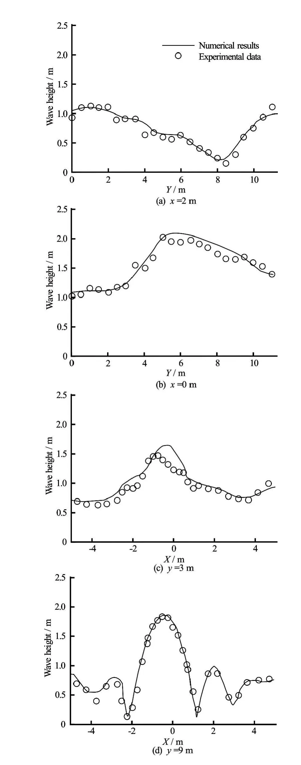
Fig.6 Wave deformation by an elliptic shoal.Comparison of the wave heights along sections

The numerical results are compared with the experimental results obtained by Synolakis[41]. The experimental test consists in the propagation of a solitarywave in a one-dimensional channel with a slope beach and it is for this that is able to verify the capacity of the numerical model to correctly represent the breaking, the run-up and the wetting-drying phenomena[42]. The numerical test is made by using a spatial discretization step of 0.05 m and a time step of 0.005 s. 475 horizontal cells and only four vertical layers are used. The beach slope is 1/20 and the waves are generated on the left boundary which is 3m far from the toe of the beach. The still water depth is 0.29 m while the wave amplitude is 0.0812 m.

Fig.7 Wave deformation by an elliptic shoal.Three-dimensional instantaneous wave field

In Fig.8 the comparison between numerical and experimental results of the free surface elevation is shown. The free surface elevation (normalized by still water depth) obtained with the numerical model is compared with the free surface elevation at different times. From Figs.8(a)-8(b)it is possible to notice how the wave profile is modified by the bottom slope interaction: the wave front becomes steeper and the breaking starts (Fig.8(c)), afterward the wave profile becomes strongly asymmetric and the wave height gradually decreases (Fig.8(d)). From Figs.8(e)-8(f)it is possible to see the maximum level of the run-up and rundown. The numerical results are in good agreement with the experimental results.

3.5 Vortices formation dues to wave-structure interaction

Fig.8 Solitary wave on a slope beach.Comparison of the free surface elevation at different time steps

Fig.9 Vortices formation due to wave-structure interaction. Sketch of the 2-layer sigma-coordinate system for the submerged structure

The resultant equations of motion for the 2-layer sigma-coordinate system are the same as those given in Section 2 by Eq.(12)and Eq.(19). The metric term expressions for the 2-layer sigma-coordinate system are given by

In Figs.10-18 the velocity field and the free surface elevation related to the wave-structure interaction are shown at different time steps. As is known, the interaction between the wave motion and the submerged obstacle can generate vortex structure[43]. In Fig.10 the free surface elevation and the velocity field are shown when the solitary wave has not yet reached the obstacle and the velocity values are small. When the wave comes near the obstacle (Fig.11) the velocity values on the left side of the obstacle increases. Subsequently (Fig.12), when the solitary wave has reached the left side of the obstacle, a little vortex on the left shoulder of the obstacle is formed while on the right side of the obstacle the velocity continue to increase. When the peak of the wave is on the left arris of the obstacle (Fig.13) the vortex on the same arris is completely developed. The vortex behind the right arris starts to form when the peak of the wave reaches the right arris of the obstacle (Fig.14), while the vortex on the left side is increasing his dimension. From Figs.15, 16 it is possible to notice how the wave crossing strongly modifies the vortices structures. In particular, the left vortex becomes sheeted and longer, while the right vortex becomes strengthen. From Figs.17, 18 it is possible to see how the vortex on the right side of the obstacle increases and persists for quite some time even when the solitary wave is far from the submerged obstacle, which is in agreement with the results shown in Lin[43].

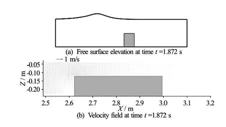
Fig.10 Vortices formation due to wave-structure interaction (t=1.872s)

Fig.11 Vortices formation due to wave-structure interaction (t=2.093s)

Fig.12 Vortices formation due to wave-structure interaction (t=2.315s)

Fig.13 Vortices formation due to wave-structure interaction (t=2.523s)

Fig.14 Vortices formation due to wave-structure interaction (t=2.709s)

Fig.15 Vortices formation due to wave-structure interaction (t=2.889s)

Fig.16 Vortices formation due to wave-structure interaction (t=3.048s)

Fig.17 Vortices formation due to wave-structure interaction (t=3.219s)

Fig.18 Vortices formation due to wave-structure interaction (t=3.303s)

3.6 Three-dimensional simulation of flow-structure interaction

Fig.19 Three-dimensional simulation of flow-structure interaction. Velocity field at timet=5s

Fig.20 Three-dimensional simulation of flow-structure interaction. Velocity field at timet=10s

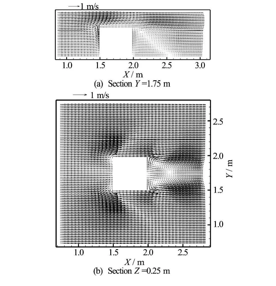
Fig.21 Three-dimensional simulation of flow-structure interaction. Velocity field at timet=15s

A Smagorinsky sub grid sub scale model is used in order to evaluate the energy dissipation related to the flow-structure interaction.

In Figs.19-21 the velocity field at three different time steps is shown. In Fig.19 the hydrodynamic flow field after 5 s is shown where unsteady condition are still in progress: from Fig.19(a)it is possible to see how a small vortex is forming downstream the upper arris and in Fig.19(b)two circulations with vertical axis are shown.

In Fig. 20 the hydrodynamic flow field after 10 s of simulation is shown: from Fig.20(a)it can be noticed that the main vortex increases its size while from Fig.20(b)it can be noticed that the axes of the horizontal vortices move in the downstream direction.

Table 1 Three-dimensional simulation of flow-structure interaction.Comparison between numerical and experimental results of the reattachment length

The value of the velocity field becomes steady after 15 s of simulation (Fig.21): the main vortex behind the obstacle is completely developed (Fig.21(a)) and the vortices with the horizontal axes have completely change their attitude. Such result is in good agreement with the one numerically produced by Li and Zhu[44]and with the experimental studies on the flow topology around prismatic obstacles with square cross section placed in a channel flow conducted by Martinuzzi and Tropea[45]. In particular, from Fig.21(b) it can be noticed that the proposed model is capable of reproducing, in terms of both its position and magnitude, the two vortices with the vertical axes downstream of the cube shown in Martinuzzi and Tropea[45]. From Fig.21(a)it can be seen that the position and the magnitude of the main horizontal axis vortex behind the obstacle is in good agreement with the experimental results of Martinuzzi and Tropea[45]and the numerical results of Li and Zhu[44]. From the same figure, it can be seen that the reattachment length of the recirculation zone downstream of the cube is(where his the size of the obstacle) which is slightly smaller than the one measured by Martinuzzi and Tropea[45]and the one numerically obtained by Li and Zhu[44]This result is coherent with the inlet velocity adopted in our numerical simulation which is half the one imposed by Martinuzzi and Tropea[45]and by Li and Zhu[44]. The comparison between the numerical and experimental results of the reattachment length is summarized in Table 1.

4. Conclusion

The proposed hydrodynamic model is based on an original integral form of the Navier-Stokes equations in a time-dependent coordinate system. The equations of motion are discretized by means of a finite-volume shock-capturing numerical procedure based on high order WENO reconstructions. The solution procedure for the equations of motion uses a third order accurate Runge-Kutta fractional-step method and applies a pressure corrector formulation in order to obtain a divergence free velocity field at each stage. In the prediction phase of the fractional-step proposed model, the equationsof motionare discretized by means of a shock-capturing numerical procedure based on high order WENO reconstructions. The numerical flux is given at each cell interface by the solution of an approximate HLL Riemann problem. As previously demonstrated the new finite-volume non-hydrostatic and shock-capturing three-dimensional model is able to simulate wave refraction, diffraction, shoaling, breaking and wave-structure interaction.

[1]Gallerano F., Cannata G. Central WENO scheme for the integral form of contravariant shallow-water equations [J]. International Journal for Numerical Methods in Fluids, 2011, 67(8):939-959.

[2]Cioffi F., Gallerano F. From rooted to floating vegetal species in lagoons as a consequence of the increases of external nutrient load, an analysis by model of the species selection mechanism [J].Applied Mathematical Modelling, 2006, 30(1):10-37.

[3]Wang B. L., Zhu Y. Q., Song Z. P. et al. Boussinesq type modelling in surf zone using mesh-less-least-square-based finite-difference method [J].Journal of Hydrodynamics, Ser. B, 2006, 18(3):89-92.

[4]Liu P. L. F., Yoon S. B., Seo S. N. et al.Numerical simulation of tsunami inundation at Hilo, Hawaii. Recent development in tsunami research [M].El-Sabh M.I. Edition,New York,USA: Kluwer Academic Publishers, 1994.

[5]Gallerano F., Cannata G., Villani M. An integral contravariant formulation of the fully nonlinear Boussinesq equations [J].Coastal Engineering, 2014, 83(1):119-136.

[6]Madsen P. A., Sørensen O. R. A new form of the Boussinesq equations with improved linear dispersion characteristics. Part 2. A slowly-varying bathymetry [J].Coastal Engineering, 1992, 18(3-4):183-204.

[7]Nwogu O. Alternative form of Boussinesq equations for nearshore wave propagation [J].Journal of Waterway, Port, Coastal, and Ocean Engineering, 1993, 119(6): 618-638.

[8]Wei G., Kirby J. T., Grilli S. T.et al. A fully nonlinear Boussinesq model for surface waves. Part 1. Highly nonlinear un steady waves [J].Journal of Fluid Mechanics, 1995, 294:71-92.

[9] Sun Z. B., Liu S. X., Li J. X. Numerical study of multidirectional focusing wave run-up of a vertical surface piercing cylinder [J].Journal of Hydrodynamics, 2012, 24(1):86-96.

[10]Fang K. Z., Zhang Z., Zou Z. L. et al. Modelling of 2-D extended Boussinesq equations using a hybrid numerical scheme [J].Journal of Hydrodynamics, 2014, 26(2): 187-198.

[11]Gallerano F., Cannata G., Lasaponara F. A new numerical model for simulations of wave transformation, breaking and longshore currents in complex coastal regions [J]. International Journal for Numerical Methods in Fluids, 2016, 80(10):571-613.

[12] Chen Q., Kirby J. T., Dalrympe R. A. et al.Boussinesq modelling of longshore currents [J].Journal of Geophysical Research Oceans, 2003, 108(C11): 156-157.

[13] Chen Q. Fully nonlinear Boussinesq-type equations for waves and currents over porous beds [J].Journal of Engineering Mechanics, 2006, 132(2):220-230.

[14] Furman D. R., Madsen P. A. Tsunami generation, propagation, and run-up with a high-order Boussinesq model [J].Coastal Engineering, 2009, 56(7):747-758.

[15]Watts P., Grilli S. T., Kirby J. T. et al.Landslide tsunami case studies using a Boussinesq model and a fully nonlinear tsunami generation model [J]. Natural Hazards and Earth System Science, 2003, 3(5):391-402.

[16] Rakha K. A., Deigaard R., Brøker I. A phase-resolving cross shore sediment transport model for beach profile evolution [J].Coastal Engineering, 1997, 31(1-4): 231-261.

[17] Johns B., Jefferson J. The numerical modelling of surface wave propagation in the surf zone [J].Journal of Physical Oceanography, 1980, 10(7):1061-1069.

[18]Casulli V., Cheng R. T. Semi-implicit finite-difference methods for three-dimensional shallow flow [J].International Journal for Numerical Methods in Fluids, 1992, 15(6):629-648.

[19] Lin P., Li C. W. A σ-coordinate three-dimensional numerical model for surface wave propagation [J]. International Journal for Numerical Methods in Fluids, 2002, 38(11):1045-1068.

[20]Lai Z., Chen C., Cowles G.et al. A non-hydrostatic version of FVCOM: 1. Validation experiment [J].Journal of Geophysical Research Oceans, 2010, 115(C11): C11010.

[21]Bradford S. F. Godunov-based model for non-hydrostatic wave dynamics [J].Journal of Waterway, Port, Coastal, and Ocean Engineering, 2005, 131(5): 226-238.

[22] Gallerano F., Cannata G.Compatibility of reservoir sediment flushing and river protection [J].Journal of Hydraulic Engineering, ASCE, 2011, 137(10):1111-1125.

[23] Ma G., Shi F., Kirby J. T. Shock-capturing non-hydrostatic model for fully dispersive surface wave processes [J]. Ocean Modelling, 2012, 43-44:22-35.

[24] Ai C., Jin S. A multi-layer non-hydrostatic model for wave breaking and run-up [J].Coastal Engineering, 2012, 62: 1-8.

[25]Fang K., Liu Z., Zou Z.Efficient computation of coastal waves using a depth-integrated, non-hydrostatic model [J]. Coastal Engineering, 2015, 97:21-36.

[26] Harlow F. H., Welch J. E. Numerical calculation of timedependent viscous incompressible flow of fluid with free surface[J]. Physics of Fluids, 1965, 8(12):2182-2189.

[27]Thomas T. G., Leslie D. C. Development of a conservative 3D free surface code [J].Journal of Hydraulic Research, 1992,30(1):107-115.

[28] Casulli V., Stelling G. S. Numerical simulation of 3D quasi-hydrostatic free surface flows [J].Journal of Hydraulic Engineering, ASCE, 1998, 124(7):678-686.

[29]Phillips N. A. A coordinate system having some special advantages for numerical forecasting [J].Journal of Meteorology, 1957, 14:184-185.

[30] Toro E. Shock-capturing methods for free-surface shallow flows [M].Manchester , UK: John Wiley and Sons, 2001.

[31]Gallerano F., Cannata G., Tamburrino M. Upwind WENO scheme for shallow water equations in contravariant formulation [J].Computers and Fluids, 2012, 62:1-12.

[32] Harten A., Lax P., Van Leer B. On upstream differencing and Godunov-type schemes for hyperbolic conservation laws [J].SIAM Review, 1983, 25(1):35-61.

[33]Trottemberg U., Oosterlee C. W., Schuller A. Multigrid [M].New York, USA: Academic Press, 2001.

[34]Stelling G., Zijlema M. An accurate and efficient finite-difference algorithm for non-hydrostatic free-surface flow with application to wave propagation [J].International Journal for Numerical Methods in Fluids,2003, 43(1):1-23.

[35] Gottlieb S., Ketcheson D. I., Shu C. W. High order strong stability preserving time discretization [J].Journal of Scientific Computing, 2009, 38(3):251-289.

[36] Spiteri R. J., Ruuth S. J. A new class of optimal high-order strong-stability-preserving time discretization methods [J]. SIAM Journal on Numerical Analysis, 2002, 40(2): 469-491.

[37] Rosenfeld M., Kwak D., Vinokur M. A fractional step solution method for the unsteady incompressible Navier-Stokes equations in generalized coordinate systems [J]. Journal of Computational Physics, 1991, 94:102-137.

[38]Zijlema M., Stelling G., Smit P. SWASH:An operational public domain code for simulating wave fields and rapidly varied flows in coastal waters [J].Coastal Engineering, 2011, 58(10):992-1012.

[39] Beji S., Batties J. A. Experimental investigation of wave propagation over a bar [J].Coastal Engineering, 1993, 19(1-2):151-162.

[40]Berkhoff J. C. W., Booy N., Radder A. C. Verification of numerical wave propagation models for simple harmonic linear water waves [J].Coastal Engineering, 1982, 6(3): 255-279.

[41] Synolakis C. E. The runup of solitary waves [J].Journal of Fluid Mechanics, 1987, 185:523-545.

[42]Gallerano F., Cannata G., Lasaponara F. Numerical simulation of wave transformation, breaking and run-up by a contravariant fully nonlinear Boussinesq equations model [J].Journal of Hydrodynamics, 2016, 28(3):379-388.

[43] Lin P. A multiple layer σ-coordinate model for simulation of wave-structure interaction [J].Computers and Fluids, 2006, 35(2):147-167.

[44]Li C. W., Zhu B. A σ-coordinate 3D k-εmodel for turbulent free surface flow over a submerged structure [J]. Applied Mathematical Modelling, 2002, 26(12):1139-1150.

[45] Martinuzzi R., Tropea C. The flow around surfacemounted, prismatic obstacles placed in a fully developed channel flow [J].Journal of Fluids Engineering, 1993, 115(1):85-92.

(Received September 10, 2016, Revised March 27, 2017

*Biography:Francesco Gallerano(1953-), Male, Ph. D., Professor

Giovanni Cannata,

E-mail: iovanni.cannata@uniroma1.it