On the clean numerical simulation (CNS) of chaotic dynamic systems ＊

Shi-jun Liao（廖世俊）

State Key Laboratory of Ocean Engineering, Shanghai Jiao Tong University, Shanghai 200240, China

MOE Laboratory of Scientific and Engineering Computing, Shanghai Jiao Tong University, Shanghai 200240,China

School of Naval Architecture, Ocean and Civil Engineering, Shanghai Jiao Tong University, Shanghai 200240,China, E-mail: sjliao@sjtu.edu.cn

On the clean numerical simulation (CNS) of chaotic dynamic systems＊

Shi-jun Liao（廖世俊）

State Key Laboratory of Ocean Engineering, Shanghai Jiao Tong University, Shanghai 200240, China

MOE Laboratory of Scientific and Engineering Computing, Shanghai Jiao Tong University, Shanghai 200240,China

School of Naval Architecture, Ocean and Civil Engineering, Shanghai Jiao Tong University, Shanghai 200240,China, E-mail: sjliao@sjtu.edu.cn

According to Lorenz, chaotic dynamic systems have sensitive dependence on initial conditions (SDIC), i.e., the butterfly-effect: a tiny difference on initial conditions might lead to huge difference of computer-generated simulations after a long time. Thus, computer-generated chaotic results given by traditional algorithms in double precision are a kind of mixture of “true”(convergent) solution and numerical noises at the same level. Today, this defect can be overcome by means of the “clean numerical simulation” (CNS) with negligible numerical noises in a long enough interval of time. The CNS is based on the Taylor series method at high enough order and data in the multiple precision with large enough number of digits, plus a convergence check using an additional simulation with even smaller numerical noises. In theory, convergent (reliable) chaotic solutions can be obtained in an arbitrary long (but finite) interval of time by means of the CNS. The CNS can reduce numerical noises to such a level even much smaller than micro-level uncertainty of physical quantities that propagation of these physical micro-level uncertainties can be precisely investigated. In this paper, we briefly introduce the basic ideas of the CNS, and its applications in long-term reliable simulations of Lorenz equation, three-body problem and Rayleigh-Bénard turbulent flows. Using the CNS, it is found that a chaotic three-body system with symmetry might disrupt without any external disturbance, say, its symmetry-breaking and system-disruption are “self-excited”, i.e., out-of-nothing. In addition, by means of the CNS, we can provide a rigorous theoretical evidence that the micro-level thermal fluctuation is the origin of macroscopic randomness of turbulent flows. Naturally, much more precise than traditional algorithms in double precision, the CNS can provide us a new way to more accurately investigate chaotic dynamic systems.

Chaos, reliable numerical simulation, clean numerical simulation (CNS), three-body problem, turbulence, origin of randomness

Prof.-Dr. Shi-jun Liao gained his Ph. D. in 1992 from Shanghai Jiao Tong University, one of the top universities in China. Thereafter, he worked in School of Naval Architecture, Ocean and Civil Engineering,Shanghai Jiao Tong University, as a Lecturer (1992),Associate Professor (1993), Full Professor (1996),Distinguished Professor of Ministry of Education of China (2 000), and “Chun shen ” Cha ir Professor (2015).

Hisresearchfieldsarefluidmechanics,chaos,computational methods and applied mathematics.

Prof. Liao is the founder of the homotopy analysis method (HAM), an analytic approximationmethod for nonlinear problems, which is now widely used by lots of researchers. Unlike perturbation techniques, the HAM is independent upon physical small parameters at all. Besides, different from all other analytic approximation methods, the HAM provides a convenient way to guarantee convergence of solution series. Thus, the HAM overcomes nearly all defects of previous analytic approximation methods. In addition,Prof. Liao proposed the “clean numerical simulation”(CNS) for chaotic dynamic systems in 2009, which can provide convergent (reliable) simulations of chaotic dynamic systems in an arbitrary long (but finite) interval of time with negligible numerical noises. As a founder of the HAM, Dr. Liao published his 1stmonograph “Beyond Perturbation: An Introduction to the Homotopy Analysis Method” in 2003 via CRC Press in USA, his 2ndmonograph “Homotopy Analysis Method in Nonlinear Differential Equations”in 2012 via Springer and Higher Education Press, and edited the book “Advances in the Homotopy Analysis Method” in 2013 via World Scientific. Prof. Liao published about 140 journal articles, with SCI citation 7329 and h-index 41. Prof. Liao was awarded“Shanghai First-class Prize for Natural Science” and“Shanghai Peony Prize for Natural Science” in 2009,and “Second Prize for National Natural Science” in 2016. He was listed three-times among “the Highly Cited Researcher” and “The World's Most Influential Scientific Minds” by Thomson Reuters in 2014 (in the fields of mathematics and engineering), 2015 and 2016 (in the field of mathematics). For more information, please visit his homepage:http://numericaltank.sjtu.edu.cn

Introduction

The famous three-body problem[1]can be traced back to Isaac Newton in 1680s. In 1890 Poincaré[1]pointed out in mathematics that trajectories of threebody problem are not integrable in general, and besides a tiny variation of initial conditions might lead to considerably obvious difference of trajectories for a long time, i.e., the sensitive dependence on initial condition (SDIC). In 1963 Lorenz[2]rediscovered the SDIC of a deterministic nonlinear dynamic system numerically by a computer, and gave it a more popular name “the butterfly-effect”: a hurricane in North America might be created by the flapping of the wings of a distant butterfly in South America several weeks earlier. Their excellent works[1,2]are milestones in science, which broke a new research field of nonlinear dynamics, say, chaos, named by Li and Yorke[3]in 1975. The chaotic dynamics[4-7]is widely regarded as the third great scientific revolution in physics in 20th century, comparable to the relativity and the quantum mechanics.

Nowadays it is well-known[4-7]that, due to the SDIC and the so-called “butterfly-effect”[2], a tiny difference in initial condition of a chaotic dynamic system enlarges exponentially. This characteristic of chaos is measured by the so-called (maximum)Lyapunov exponent. In theory, the (maximum)Lyapunov exponent of a chaotic dynamic system must be positive[4-7].

Nowadays, high performance computers are widely used to gain numerical simulations of nonlinear differential/integral equations. Unfortunately,numerical noises, i.e., truncation error and round-off error, are always unavoidable for any numerical simulations. Many people believe that convergent(reliable) numerical simulations would be obtained as long as temporal and spatial discretizations are fine enough. This is true for many nonlinear equations but unfortunately not for chaotic systems. As pointed out by Lorenz[8], a chaotic system is sensitive not only to initial conditions but also to numerical algorithms: the(maximum) Lyapunov exponent of a chaotic model always alters between negative and positive values even when the time-step becomes rather small[8]. It means that the basic characteristic of the corresponding numerical simulations changes alternately between periodic and chaotic, which however are fundamentally different from each other. From such kind of numerical simulations, it is even impossible to determine whether it is a chaotic system or not. Such kind of numerical phenomenon was confirmed by many others. For example, Teixeira et al.[9]investigated the time step sensitivity of three nonlinear atmospheric models by means of traditional algorithms in double precision, and made a pessimistic conclusion that, “for chaotic systems, numerical convergence cannot be guaranteed forever”, and that “for regimes that are not fully chaotic, different time steps may lead to different model climates and even different regimes of the solution”. In 2015 Hoover et al.[10]illustrated the Lyapunov's instability by comparing numerical simulations of a chaotic Hamiltonian system given by two Runge-Kutta and five symplectic integrators in double precision, and found that “all numerical methods are susceptible to Lyapunov instability, which severely limits the maximum time for which chaotic solutions can be accurate”, although“all of these integrators conserve energy almost perfectly” and “they also reverse back to the initial conditions even when their trajectories are inaccurate”.As reported by Hoover and Hoover[10], “the advantages of higher-order methods are lost rapidly for typical chaotic Hamiltonians”, and “there is little distinction between the symplectic and the Runge-Kutta integrators for chaotic problems, because both types lose accuracy at the very same rate, determined by the maximum Lyapunov exponent.”

Even for some nonlinear dynamical systems without Lyapunov's instability, it is rather hard to gain accurate prediction, too. Li et al.[11]studied the sensitive dependence of the fixed point of Lorenz equation (in a case without chaos) on the time-step by means of many explicit/implicit numerical approaches(such as Euler's method, the Runge-Kutta methods at orders from 2 to 6, Taylor series methods at orders from 2 to 10, Adams methods at orders from 2 to 6,and so on) in double precision, but found that the long-term numerical simulations are rather sensitive to the step size, say, they always fluctuate between the two fixed points, no matter how small the time-step is.Thus, Li et al.[11]made a pessimistic conclusion that“numerical solution obtained by any step sizes is unrelated to exact solution”.

These numerical phenomena cast a shadow and lead to some serious doubts on the reliability of numerical simulations of chaos. Naturally, some intense arguments[12,13]are unavoidable. For example, Yao and Hughes[12]believed that “all chaotic responses are simply numerical noise and have nothing to do with the solutions of differential equations”. Yao[14]even believed that “reports of computed non-periodic solutions of chaotic differential equations are simply consequences of unstably amplified truncation errors,and are not approximate solutions of the associated differential equations”.

This shadow becomes a dark cloud over the blue sky of chaos, which presents a great challenge for us.Canwe gainconvergent (reliable)numerical simulations of chaotic dynamic systems in along enough interval of time?

In history of science, challenge and chances always coexist. The above-mentioned intense arguments[12-14]lead the author to think deeply about the essence of chaos, and as a result to put forward a numerical approach, namely the “clean numerical simulation” (CNS)[15-21], which can sweep this dark cloud away. By means of the CNS, the numerical noises can be so greatly reduced that they are negligible (compared to all physical variables under investigation) even in an arbitrary long (but finite)interval of time. For example, the convergent (reliable)numerical simulations of chaotic solution of Lorenz equation in a rather long interval [0,10000] were gained by means of the CNS, for the first time[18].Besides, numerical noises of the CNS can be much smaller even than micro-level physical uncertainty so that, using the CNS, we can provide a rigorous theoretical evidence that the micro-level physical thermal fluctuation is the origin of the macroscopic randomness of Rayleigh-Bénard turbulent flows[20]. In addition, the CNS has been successfully applied to find hundreds of new periodic orbits of three-body system[21], a famous classical problem that can be traced back to Isaac Newton in 1680s. These new periodic orbits have never been reported before, which therefore illustrate the great potential of the CNS.

In this paper, we will briefly describe the strategy and basic ideas of the CNS, its applications in Lorenz equation, three-body problem, Rayleigh-Bénard turbulent flows, and so on.

1. Basic ideas of the CNS

Almost all chaotic dynamic systems are numerically solved by computers. This unavoidably leads to numerical noises, i.e., truncation and round-off errors.For simplicity, let us consider the th-M order Taylor expansion of a real function

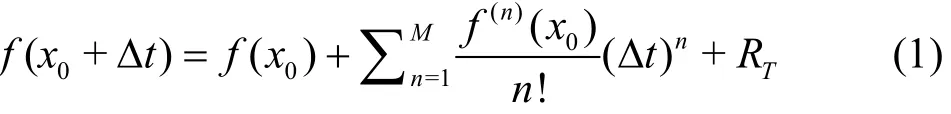
where Δt is the time step, f(n)() is the nth-order derivative of f(x) at x0, RTis the truncation error, respectively. When the time step Δt is within the convergence radius, the larger the order M, the smaller the truncation error RT, so that RT→ 0 as M → ∞ . The round-off error is due to the limited precision of data expressed by a finite number of digits. Both of the truncation error and round-off error belong to the so-called “numerical noises”, which are unavoidable to any numerical computations. For high performance computer, the truncation error can be reduced to any a required level by means of large enough order M of Taylor series. Besides, the round-off error can be reduced to any a required level by means of the so-called multiple-precision (MP)data[22]with a large enough number of digits, which,for example, can be used to calculate π in accuracy of millions of digits.

The CNS[15-21]is a new strategy for reliable simulations of chaos, which is based on the Taylor series method[23-27]at high enough order of approximation and the use of data in MP[22]with large enough number of digits, plus a convergence (reliability)check of computer-generated simulations by means of an additional computation with even smaller numerical noises. The Taylor series method[23-27]is one of the oldest method, which can be traced back to Newton,Euler, Liouville and Cauchy. It has such an obvious advantage that its formula at arbitrary order can be expressed in the same form. So, from numerical viewpoint, it is rather easy to use the Taylor series method even at very high order so as to deduce truncation error to any a required level. Besides, the round-off error can be reduced to arbitrary level by means of either computer algebra system (such as Mathematica, Maple and so on) or the MP library[22].In summary, the CNS uses the following strategies:

(1) Reduce the truncation error to a required tiny level by means of Taylor series expansion at large enough order M for all unknown functions.

(2) Reduce the round-off error to a required tiny level by expressing all data (including all unknown functions, physical parameters, temporal and spatial discrete sizes, and so on) in multiple precision using many enough digits.

(3) Check the convergence (reliability) of numerical results by means of comparing two simulations given by Taylor series expansion at different orders,and/or multiple-precision data in different numbers of digits, and/or different temporal and spatial discrete sizes.

The strategies of the CNS are very simple in mathematics and rather easy-to-use in practice by means of high performance computers. These strategies are mainly based on the great advance in computer science and high technology in computer industries. Briefly speaking, the CNS reduces the numerical noises so greatly that they are much smaller than physical unknown variables under investigation and thus become negligible even in a long interval of time.Note that the convergence (reliability) check by means of comparing two different simulations at different levels of numerical noises is widely used in the field of uncertainty quantification[28]. In fact, each strategy of the CNS has been used separately for different purposes by many researchers. Here, we combine them as a whole to gain convergent (reliable) numerical simulation of chaotic dynamic systems in a long enough interval of time.

In the next section, the famous Lorenz equation will be used to illustrate how to gain convergent(reliable) numerical simulations of a chaotic dynamic system in a long enough interval of time by means of the CNS.

2. Long-term reliable simulation of chaos by CNS

Without loss of generality, let us consider a simple model for weather forecast used by Lorenz[2],the famous Lorenz equation:

where , R, b are physical parameters, the dot denotes the differentiation with respect to the time t,respectively. We consider here a chaotic case

with the initial condition

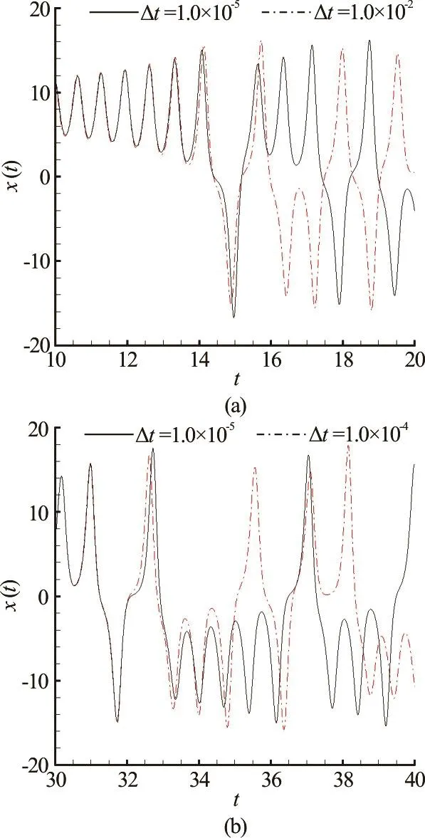
Fig.1 Sensitive dependence of numerical trajectories on the time step Δt. The trajectoriesare given by the-order Runge-Kutta's method in double precision

In the frame of the CNS, we first of all solve Eq.(2) by means of the th-M order Taylor expansions

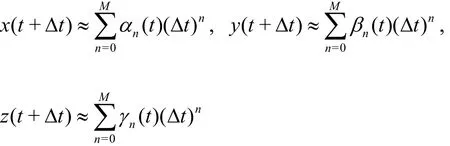
Substituting the above series into the Lorenz equation(2) and equating the like-power of the time step Δt,we have the recurrence formulas (0 ≤ n ≤ M - 1 ):

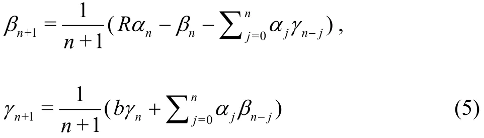
For details, please refer to Liao[15]. It is convenient to calculate these values by means of parallel computations even for quite high orderM. Thus, the truncation error can be reduced toanya required level as long as large enoughMis used.

Secondly, to reduce the round-off error, we expressalldata in -Ndigit precision by means of the MP package[22]. In this way, the round-off error can be reduced toanya required level as long as large enoughNis used.

Thirdly, the convergence (reliability) interval[0,Tc] of a numerical simulation is determined by comparing it with an additional simulation using even smaller numerical noises, i.e., by means of higher order of Taylor series, and/or more precise data with more digits, and/or smaller time step Δt.

In the frame of the CNS, it is unnecessary to choose a tiny time step. Here, we use the time step Δt=0.01 for Lorenz equations (2) and (4) in case of(3), if not mentioned particularly.

Due to the butterfly-effect of chaos, the convergence interval [0,Tc] is sensitive to both ofM(the order of Taylor series) andN(the number of digits for multiple-precision data). To investigate the influence of the order of Taylor series onTc, we use long enough MP data, say,N=max{200,2M} ,whereMis the order of Taylorseries. In this case, itis fou that the length of the convergence(reliability) interval [0,Tc] is approximately directly proportional to the orderMof Taylor series, say,

Similarly, it is found[15]that, for a properly givenM(the order of Taylor series), the convergence (reliability) interval [0,Tc] is approximately directly proportional to the precision of MP data, say,

whereNis the number of digits of the multipleprecision data. Therefore, to gain convergent (reliable)simulations of chaotic systems, we must reducebothof the truncation and round-off errors! For example, in order to gain convergent chaotic solution of Lorenz equation in [0,1000], wehadto use Taylor series at order higher than 333andthe MP data with more than 400 digits. According to (7), it is now very clear why“numericalconvergencecannotbe guaranteedforever”[9]byanyalgorithms indoubleprecision. It is indeed a pity that the importance of round-off error for chaotic dynamic systems was ignored in general[29,30].In 2009, Liao[15]successfully applied the CNS to gain a convergent chaotic solution of Lorenz equations(2)-(4) in the interval [0,1000] by means of the 400th-order Taylor series method and data in 800-digit precision, whose convergence can be confirmed by means of an additional simulation using the 420th-order Taylor series method and data in 820-digit precision.

Note that, the chaotic results given by the traditional 4th-order Runge-Kutta's method in double precision are convergent in a rathersmallinterval[0,12.5]. However, by means of the CNS, theconvergentchaotic solution in amuchlarger interval[0,1000] is obtained by Liao[15],for the first time. In mathematics, this kind of simulation given by the CNS is reliable. This is mainly because the numerical noises, i.e., both of the truncation error and round-off error, are greatly reduced to be so small that they are negligible even in such a long interval [0,1000] for a chaotic dynamic system.

Table 1 Convergen t (relia bl e) ch aotic so lution of Lo renz equatio ns (2)- (4)in thei nterval[0,1000 0]by meansoftheCNSusingthe3orderTaylor expansion, MP data in 4180-digit precision and the time step Δt=0.01

Table 1 Convergen t (relia bl e) ch aotic so lution of Lo renz equatio ns (2)- (4)in thei nterval[0,1000 0]by meansoftheCNSusingthe3orderTaylor expansion, MP data in 4180-digit precision and the time step Δt=0.01

t()xt ()yt()zt 0 -15.8000 -17.480035.6400 1 000 13.8820 19.918326.9019 2 000−6.8739-1.484831.3495 3 000 1.6933 3.600321.4109 4 000−7.6927 -13.499614.1994 5 000−6.0844−10.813712.7391 6 000 0.2167 2.104322.1246 7 000−11.3949−16.575423.6813 8 000−1.2659−2.336317.4960 9 000 13.4797 17.282129.2382 10 000 −15.8173 −17.3669 35.5584

According to (6) and (7), convergent (reliable)chaotic solutions of Lorenz equations (2) to (4) in evenlargerintervals [0,Tc] can be obtained by means of higher order Taylorseriesand morepreciseMP data. This is indeed true.In 2012, Wang successfully applied the CNS to gain convergent chaotic solution of the Lorenz equations(2) to(4)inthe interval [0,2500] by means oforder Taylor series, the MP data in 2 100-digit precision and the time step Δt=0.01, whose convergence and reliability were confirmed by an additional simulation given by the 1 200th-order Taylor series and MP data in 2 100-digit precision. In 2014, using a parallel algorithm and 1 200 CPUs on the national supercomputer TH-1A (at Tian Jian, China), Liao and Wang[18]further applied the CNS to gain the convergent(reliable) chaotic solution of the Lorenz equations (2)to (4) in a rather long interval [0,10000] by means of the 3 500th-order Taylor expansion and MP data in 4 180-digit precision, whose convergence and reliability in such a long interval [0,10000] was confirmed by an additional simulation using the 3 600th-order Taylor expansion and MP data in 4 515-digit precision!Some convergent results of the Lorenz equations (2)to (4) are given in Table 1.

Notethat,using the traditional 4th-order Runge-Kutta's method in double precision, one can gain convergent chaotic results of Lorenz equation only in a rather small interval [0,12.5], which naturally leaded to the famous conclusion “long-term prediction of chaos is impossible”. However, by means of the CNS, one can gain convergent chaotic solution of Lorenz equation in such a long interval[0,10000] that is 800 times longer than [0,12.5].Our CNS results suggest that, from the mathematical viewpoint, long-term prediction of chaos is possible.Therefore,convergent numericalsimulationsof chaotic systems indeed exist, which are neither“simply numerical noise”[12]nor “simply consequences of unstably amplified truncation errors”[14],and thus should have something to do with the solutions of the corresponding differential equations.The reason of their pessimism in Refs.[9,12,14] is mainly the use of double precision. So, unlike Teixeira et al.[9], Yao and Hughes[12]and Yao[14], the author is rather optimistic on the reliability of longterm simulations of chaotic dynamic systems. This kind of optimism is based on our convergent (reliable)chaotic results of Lorenz equation in such a long interval of time! Hopefully, these convergent chaotic results[18]in the interval [0,10000] given by the CNS could quiet down the intense arguments[9,12-14],and might deepen our understandings and enrich our knowledge about chaotic dynamic systems.

It is interesting that the advance in computer science and industry greatly promotes the development of chaotic dynamics as a scientific research field.Although the SDIC was first found by Poincaré in 1890 (mainly from mathematical viewpoint), it is Lorenz who made the SDIC rather popular in scientific community (with a more popular name “butterflyeffect”) by means of numerically solving the so-called Lorenz equation using the 4thorder Runge-Kutta's method in double precision on a computer in 1963.In 1960s the performance of computer was poor and the multiple-precision package did not exist, thus naturally one might make the conclusion that“long-term prediction of chaos is impossible”.Nowadays, with the high-performance supercomputers and the multiple-precision data, long-term prediction of chaos becomes possible (from mathematical viewpoint) at least by means of the CNS!

Naturally, with negligible numerical noises in such long intervals of time, the CNS provides us a new way to more precisely investigate chaotic dynamic systems in more details. Some examples are given below.

3. Some applications of the CNS

The CNS has been successfully used to solve many chaotic dynamic systems in long enough (but finite) interval of time. Here, a few examples are given to illustrate the potential and validity of the CNS.

3.1 Reliable numerical simulations of a chaotic threebody system

The famous three-body problem[1]can be traced back to Isaac Newton in 1680s. As pointed out by Poincaré[1], three-body problem is generally unintegrable and has SDIC, i.e., the butterfly-effect of chaos[2]. Similarly, convergent (reliable) numerical simulations of chaotic three-body systems in a long enough interval of time can be gained by means of the CNS, as long as one has enough resources of computation.

Without loss of generality, let us consider the famous three-body problem governed by Newtonian gravitational law with the dimensionless equations

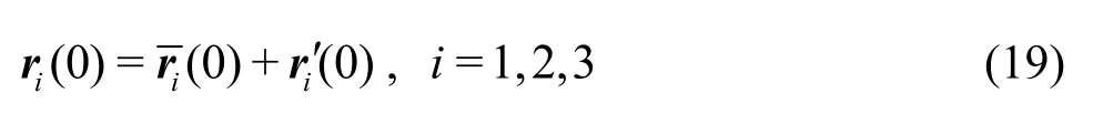
where ri=(x1,i, x2,i, x3,i)denotes the dimensionless position of the it h -body, ρi= mi/m1is the ratio of mass (i = 1,2,3), with the definition

For simplicity, we consider here the case ρ1= ρ2= ρ3= 1. Let us consider the zero-momentum initial conditions

and

As mentioned by Sprott[7](Fig.6.15, pp. 137), the three-body problem (8) with the initial conditions (9)and (10) is chaotic, with the maximum Lyapunov exponent λ= 0.1681. Thus, the corresponding numerical noises enlarge exponentially.

In the frame of the CNS, the motion equationto the initialconditionsand (10) was solvedbyinalongenough intervalby means of the M t h -order Taylor series and the MP data in 300-digits precision. For detailed mathematical formulas, please refer toSince each data is expressed in 300-digit precision, the round-off error is rather small (compared to the physical uncertainty considered later in Section 3.2) and thus negligible. In addition, the higher the order M of Taylor expansion is, the smaller the truncation error is and the more accurate the results at t = 1000 are. Assume that, at t = 1000, we have the result x1,1= 1 .8151 0 12345 by means of the M1t h-order Taylor expansion and the result x1,1= 1 .81510 47535 by means of the M2thorder Taylor expansion, respectively, where M2＞M1. Then, the result by means of the M1thorder Taylor expansion is said to be in the accuracy of 5 significance digit, expressed by ns=5.

It is found by Liao[17]that the CNS simulations using the time step =0.01tΔ and Taylor series at the 8th, 16th, 24th, 30th, 40thand 50thorders agree each other in the whole interval [0,1000] in the accuracy of 11,23, 38, 48, 64 and 81 significance digits, respectively.Approximately,sn, the number of significance digits of the positions at =1000t , is linearly proportional to M (the order of Taylor expansion), say,

For example, the CNS simulation using the 50th-order Taylor expansion and data in 300-digit precision (with the time step =0.01tΔ) provides us the position of Body-1 at =1000t in the accuracy of 81 significance digit:

Besides, it is found by Liao[17]that, using the smaller time step Δ t =0.001 and the MP data in 300-digit precision, the CNS simulations given by the 8th, 16th, 24thand 30thorder Taylor expansion agree in the whole interval [0,1000] in the accuracy of 18, 38,62 and 77 significance digits, respectively. Approximately, ns, the number of significance digits of the positions at t = 1000, is linearly proportional to M(the order of Taylor expansion), say,

It should be emphasizedthat the CNS simulationsgiven by the time step Δ t =0.001 and the-order Taylor series (M = 30) agree in the accuracy of the 77 significance digits with those by the time stepΔ t =0.01 and the -order Taylor seriesin the whole interval [0,1000].

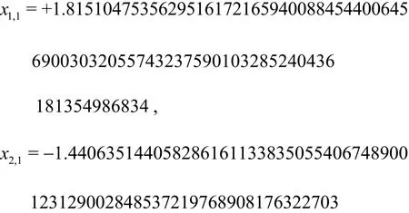
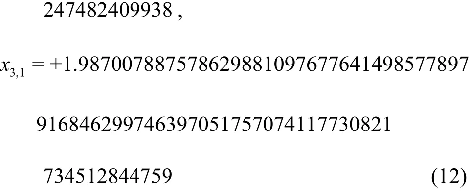
In addition, the momentum conservation is satisfied in the level of 10-295. All of these confirm the mathematical correction and reliability of our CNS simulations. Thus, although the considered three-body problem has chaotic orbits, we are quite sure that our numerical simulations given by the CNS using the 50th-order Taylor expansion and the MP data in 300-digit precision (with the time step =0.01tΔ) are mathematically reliable in the accuracy of 77 significance digits in the whole interval 01000t≤≤. These CNS results are rather precise, even compared to the micro-level physical uncertainty investigated later in Section 3.2. The corresponding convergent orbits of the three bodies are as shown in Fig.2. Note that the orbits of Body-1 and Body-3 are chaotic, but Body-2 oscillates along a line on the plane =0z . Note that we have the zero-momentum initial conditions (9) and (10). So,due to the momentum conservation, the chaotic orbits of Body-1 and Body-3 are symmetric about the regular orbit of Body-2. Thus, although the orbits of Body-1 and Body-3 are disorderly, the three-body system as a whole has an elegant symmetry. In the following section, we will show that such kind of elegant symmetry might break without any external disturbance, say, out-of-nothing!

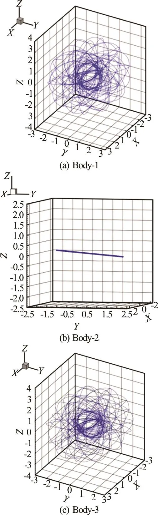
Fig.2 Orbits of th e three -body syst em (8) subject to the zero- mo me ntuminitialc onditi ons (9) and(10 ) in the accuracy of77significancedigitsinthewholeinterval 0≤t≤ 1000, given by m eans of the CNS using the -or der Taylorseriesanddatain300-digitprecisionwiththe time-step Δt=0.01

3.2 Origin of inherent macroscopic randomness of chaotic three-body system

When one looks at the sky in a clear night, he/she might feel that stars seem to distribute randomly.Besides, it is well-known that measured velocities in turbulent flows are always different at the same places of observation even using the same equipment by the same people in the same lab. Indeed, random/uncertain macroscopic phenomena happen quite frequently in practice. However, what is the originof macroscopic randomness (uncertainty)? This is one of the most fundamental questions in science. Without doubt,the answers to this open question might greatly deepen our understandings and enrich our knowledge about nature.

With negligible numerical noises in arbitrary long (but finite) intervals, the CNS provides us a useful tool to precisely investigate the propagation of physical micro-level uncertainties, which can give us a rigorous theoretical evidence about the origin of the macroscopic randomness and the symmetry-breaking of three-body system, as shown below.

For example, let us consider the three-body system (8) in case of ρ1= ρ2= ρ3= 1. Note that the convergent (reliable) chaotic trajectories are obtained in a long enough interval [0,1000] in accuracy of 77 significance digits by means of the CNS using the 50th-order Taylor series, the MP data in 300-digit precision and the time step Δt=0.01. The numerical noises are so small that even the physical micro-level uncertainty could be investigated precisely, as mentioned below.

Note that the initial conditions (9) and (10) used in Section 3.1 are mathematically exact, say, in accuracy of 300-digit precision. However, this is impossible physically. In physics, the Planck length

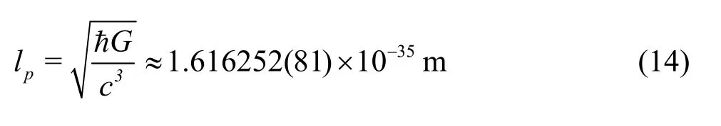
is the length scale at which quantum mechanics,gravity and relativity all interact very strongly, where c is the speed of light in a vacuum, and G is the gravitational constant, respectively. According to the string theory[32], the Planck length is the order of magnitude of oscillating strings that form elementary particles, and shorter lengths do not make physical senses. Especially, in some forms of quantum gravity,it becomes impossible to determine the difference between two locations less than one Planck length apart. Therefore, in the level of the Planck length,position of a body is inherently uncertain. This kind of microscopic physical uncertainty is inherent and has nothing to do with Heisenberg uncertainty principle[33],say, it is objective.

In addition, according to de Broglie[34], any a body has the so-called wave-particle duality. The de Broglie's wave of a body has non-zero amplitude.Thus, position of a body is uncertain: it could be almost anywhere along de Broglie's wave packet. So,according to de Broglie's wave-particle duality,position of a star/planet is also inherent uncertain, too.Therefore, from the physical viewpoint, the microlevel inherent fluctuation of position of a body shorter than the Planck length (14) is essentially uncertain and/or random.

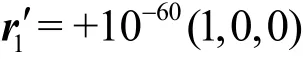
Therefore, let us further consider the three-body system (8), subject to the same initial velocities (10)but the initial positions with physical micro-level uncertainty

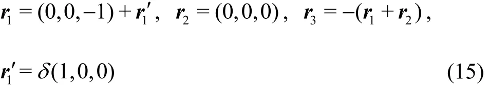
where δ is a constant to be given later. To make the Planck length lpdimensionless, we use the diameter of Milky Way Galaxy as the characteristic length, say,dM=105light year ≈ 9 × 1 020m . Note that

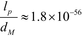
is a rather small dimensionless number. So, as mentioned above, two (dimensionless) positions of the three-body system shorter than 1.8×10–56do not make physical senses in physics. So, it is reasonable to assumethat the inherent uncertainty of the dimensionless position of the three-body systems in(15) is in the micro-level 10-60, say, either δ = +10-60or δ =-1 0-60,which are even lessthan≈ 1 .8× 1 0-56a few orders of magnitude.It shouldbe emphasized again that, according to the stringtheory[32],thetiny physical uncertainty∓ 10-60(1,0,0)of the initial positions (15) is so small that all of th ese initial conditions are the same inphysics,nomatter either δ =+10-60or δ=-10-60or δ=0.

Mathematically, δ =∓1 0-60is a tiny number,which however is much smaller than numerical noises of traditional algorithms in double precision. So, it is impossible to precisely investigate the influence and propagation of this inherent micro-level uncertainty of initial conditions by means of traditional numerical methods in double precision. However, the microlevel uncertainty δ = ∓1 0-60is much larger than the numerical noises of the CNS using the Taylor series method at high enough order and the MP data in 300-digit precision with a reasonable time step, as illustrated below.

For example, the position of Body-1 at t =1000 given by the CNS using the 50th-order Taylor series method and the MP data in 300-digit precision with the time step Δ t =0.001 reads to M(the order of Taylor expansion), say,

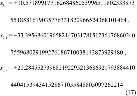
which are in the accuracy of 72 significance digits,with the zero-momentum conservation satisfied at the level of 10-293. Thus, our CNS simulation in case of δ=+10-60is mathematically convergent (reliable) in the whole interval [0,1000]. However, the positions(17) of the three-bodies at =1000t in case of δ=+10-60are quite different from those (12) in case of =0δ, as shown in Figs.2 and 3.

It is found that, within 0810t≤≤, the chaotic orbits of the three bodies are not obviously different from those in the case of =0δ, say, Body-2 oscillates along the same line on the plane =0z ,Body-1 and Body-3 are chaotic with the symmetry about the Body-2. However, the obvious difference of orbits appears when 810t＞ : Body-2 escapes together with Body-3 along a complicated threedimensional orbit, while Body-1 escapes in an opposite direction. As shown in Fig.3, Body-2 and Body-3 depart far and far away from Body-1and finally become a binary-body system. It is very interesting that, when 810t＞ , the tiny physical uncertainty

of the initial conditions disrupts not only the elegant symmetry of the orbits but also even the three-body system itself. In other words, this tiny physical uncertainty leadstothemacroscopicobvious difference of orbits after 810t＞ .

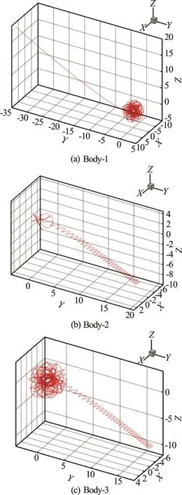
Fig.3 Orbits of the three-body system (8) subject to the zero- momentum initial conditions (10) and (15) in case of δ= + 1 0-60in the accuracy of 72 significance digits in the whole inte rval 0≤t ≤1000 , given by mean s o f the CNS usingthe50th-orderTaylorseriesanddatain300-digit precision with the time-step Δ t =0.001

Similarly, in the case ofδ= -1 0-60, we gain the convergent (reliable) orbits of the three bodies on the whole interval [0,1000] by means of the CNS using the time step Δt=0.001, the MP data in 300-digit precision and the 20th-order Taylor expansion. As shown in Fig.4, the tiny physical uncertainty in the initial position disruptsnotonly the elegant symmetry of the orbitsbutalso the three-body system itself as well: whent＞ 8 10, Body-2 escapes (this time with Body-1) in a complicated three-dimensional orbit,while Body-1 and Body-3 departs in two opposite directions without any symmetry. Note that, in the case ofδ=-1 0-60, Body-2 and Body-1 depart far and far away from Body-3 to finally become a binary system. Note that, in the case ofδ= +10-60, Body-2 and Body-3 escape together to become a binary system! This is very interesting. Thus, the chaotic orbits of the three-body system subject to the initial conditions (15) with the micro-level physical uncertainty, corresponding toδ=0,δ=+10-60andδ=- 1 0-60, respectively, are completely different whent＞ 8 10. However, it should be emphasized that,thesemathematicallydifferent initial conditions arephysicallythesame, since any spatial differences shorter than the Planck lengthdonotmake physical senses, due to the string theory[32].

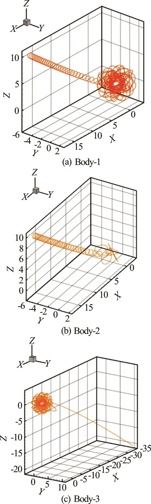
Fig.4 Orbits of the three-body system (8) subject to the zero- momentum initial conditions (10) and (15) in case of δ= - 1 0-60 in the whole interval 0≤t≤1000, given by means of the CNS using the 20th-order Taylor series and data in 300-digit precision with the time-step Δ t =0.001

To check the generality of the above-mentioned results, we further consider the three-body system (8)with the same initial velocity (10) but the initial position condition with a different tiny physical uncertainty

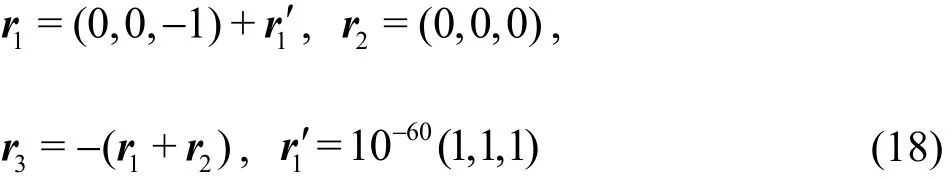
Fig.5 Orbits of t he thre e-body sys tem ( 8) s ubjec t to the zero- momentuminitialconditions(10)and(18)inthewhole interval 0≤t≤1200, given by means of the CNS using the 30th-order Taylor series and data in 300-digit precision with the time-step Δ t =0.001

Similarly, the corresponding convergent (reliable)orbits in the interval [0,1200] are obtained by means of the CNS using the 30th-order Taylor series method and the MP data in 300-digit precision with the time step Δ t =0.001. It is found that, in the interval 0≤t≤810, the orbits are almost the same as those given in case of the initial conditions (9) and (10), but beyond it they become quite different from those in the above-mentioned three cases: Body-2 escapes(with Body-3) along a complicated three-dimensional orbit, while Body-1 and Body-3 depart from each other in two opposite directions, as shown in Fig.5.This confirms our previous conclusions.

Then, let us consider the three-body system (8)subject to the same initial velocity condition (10) but an initial position condition in more general case, i.e.,containing a micro-level physical uncertainty,i = 1,2,3, in Gaussian normal distribution with the standard deviation σ0at the level of 10-60, say,

where

with the definitions

Note that the initial conditions (9), (15) and (18) are special cases of (19) and (20).

First of all, let us consider the case σ0=10-60.Ten thousand samples of reliable (convergent) simulations ofthe chaoticthree-body system subject to (10),(20) and (21) wereobtained by Liaoand Li[19]in the time interval [0,1000] by means of the CNS using the multiple-precision data in 300-digit precision, the time-step Δ t =0.001 and high-enough order M of Taylor series expansion, where M ≥ 3 0 in general.Each chaotic solution was verified by means of a higher-order Taylor series expansion with the same initial condition, and only convergent results in the interval [0,1000] were accepted. In this way, the man-made uncertainty is negligible, since numerical noise is much smaller than physical uncertainty in the whole interval of time. Thus, the micro-level inherent physical fluctuationof the initial position ri( 0) is the only source of uncertainty. It is found that the ten thousand orbits are almost the same within 0≤t≤810, but become quite different beyond it, as shown in Fig.6.

Similarly, in the case of σ0=3× 1 0-60, it is found that the ten th ousa nd orbits are almos t the same within0≤t≤810,butbecomesobviouslydifferent,as shown in Fig.7. It is in teresting that the prob ability/statisticdistributionoforbits withint＞ 8 10is dependent upon the standard deviation0σof microlevel physical uncertainty, as shown in Figs.6 and 7.However, at 1000t= , such kind of probabi-lity/statistic distributions given by two different standard deviations are quite similar.

Fig.6 The p osition d istri bution o f Body -1 (red poi nts) , Body-2 (greenpoints)andBody-3(bluepoints)inthe(x,y) plane at different times when σ=10-60. Results are 0 based on the 10 000 samples of convergent (reliable) simu- lat ions gi ven by th e CN S w ith th e m icro-leve l fluctuation ofini tialp osit ion(20)and (21 )inG aussiandistribution. Suchkindofdistributionhassomeprobability/statistic meaning

Fig.7 The p osition d istri bution of Body -1 (red poi nts), Body-2 (greenpoints)andBody-3(bluepoints)inthe(x,y) plane at different times when σ =3× 1 0-60. Results are 0 based on the 10 000 samples of convergent (reliable) simu- lations given by the CNS with the micro-level fluctuation of initial position (20) and (21) in Gaussian distribution

All of our convergent (reliable) simulations reveal that there exists such an intervalwhere≈ 8 10 for the considered three-body system, that the chaotic trajectories of the three bodies have no obvious difference withinbut become obviously different beyond it. It should be emphasized that, by means of the CNS with high enough order Taylor series method and the MP data in high enough precision, the numerical noises are negligible so that all chaotic trajectories are convergent (reliable) in the whole interval [0,1000]. On the other side, the micro-level physical uncertainty of positions of these initial conditions is shorter even than the Planck length so that they are the same in physics, according to the string theory[32]. However, each of these physically same (but mathematically different) initial conditionscan sample with equal probability,although we do not know which one will practically occur. Therefore, from physical viewpoint, the chaotic trajectories when t ＞are essentially uncertain,say, we cannot predict the physically correct trajectories after t ＞, forever. This provides us a new concept, i.e., “the physical limit time of prediction”, denoted by, which gives a time-scale for “at most how long a deterministic prediction of chaotic dynamic systems is physically correct”. Our ability of prediction is greatly restricted by the physical limit time of prediction, which is objective, i.e., independent of numerical methods and limited precision of measurement. The new concept, “the physical limit time of prediction”, also provides us a time scale for the micro-level, objective, physical uncertainty of chaotic systems to transfer into macroscopic randomness. The three-body system (8)-(10) provides us a good example that the micro-level physical uncertainty might be the origin of macroscopic randomness. This suggests that macroscopic randomness should have a close relationship with micro-level uncertainty and thus is essentially unavoidable. Besides, the concept of “the physical limit time of prediction” also implies that the macroscopic model of the chaotic three-body systems based on Newtonian gravitational law is essentially not deterministic, because the initial condition contains the micro-level physical uncertainty that is unavoidable and might become very important for a long time beyond.

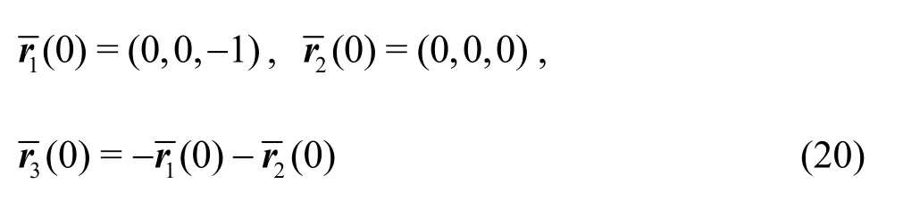
Let ε0, ε1denote the levels of physical microscopic uncertainty and macroscopic randomness,the maximum Lpayunov exponent of chaotic system,respectively. Then, it holds

which gives the relationship

This also provides us a new way to calculate the maximum Lyapunov exponent

by means of the CNS. Note that (23) might give the Lyapunov exponent a physical meaning.

The physical limit time of prediction, Tlim, has

p general meanings: it provides us a time-scale of physically correct prediction for chaos: it has no physical sense to talk about any “prediction” of chaotic trajectories beyond T plim, since they are essentially uncertain in physics. Hopefully, this concept might be helpful to deepen our understandings about chaos.

It should be emphasized that all of these 10 000 orbits have the same initial conditions in physics,since a tiny difference of position shorter than Planck length does not make physical senses, according to the string theory[32]. When t ＜ Tplim, all of these 10 000 orbits have almost the same orbits with the elegant symmetry. However, when t ＞ Tplim, these physically same initial conditions lead to the macroscopic randomness, the symmetry-breaking and the system disruption of the three-body system, without any external disturbance,i.e.,out-of-nothing! In other words,such kind of macroscopic randomness,symmetry-breaking and system disruption of the three-body system are self-excited. So, we can call them “self-excited macroscopic randomness”, “selfexcited symmetry-breaking” and “self-excited system disruption” of the three-body system.

Finally, it should be emphasized that it is the CNS that provides us a useful tool to precisely investigate such kind of propagation of micro-level physical uncertainty. This is mainly because, unlike traditional numerical algorithms in double precision,the numerical noises of the CNS can be even much smaller than the micro-level uncertainty in the whole interval of time under consideration!

3.3 Origin of intrinsic randomness of Rayleight-Bénard turbulence

It is well known that turbulent flows are random.What is the origin of such kind of randomness of turbulence? This fundamental problem remains open,to the best of our knowledge. In this section, by means of the CNS as a reliable numerical tool with negligible numerical noises, we use the two-dimensional Rayleigh-Bénard convection flow as an example to illustrate that turbulence can be self-excited from the inherent thermal fluctuation without any external disturbances, i.e., out of nothing.

External disturbances and man-made uncertainty are unavailable in any physical experiments of turbulent flows. Certainly, they draw uncertainty into turbulent flows. Are turbulent flows still random even if all of these external disturbances and man-made uncertainty do not exist? This is a fundamental question.

To avoid external disturbances and man-made uncertainty, we had to numerically solve the Navier-Stokes (N-S) equations, which are widely used to describe turbulent flows. Unfortunately, numerical noises are unavailable in any traditional algorithms in double precision. Note that the famous Lorenz equations can be derived originally from the N-S equations,whose solutions are chaotic in general and have sensitive dependence not only on initial conditions(SDIC)[2]but also on numerical algorithms[8]. So,numerical simulations of the NS equations given by traditional algorithms in double precision are a kind of mixtures of the “true solution” and numerical noises at the same level. However, using the CNS, we can reduce numerical noises to an arbitrary level so that they are much smaller than all physical quantities in a long enough interval of time. In this way, the man-made uncertainty due to numerical noises can be negligible, as described below.

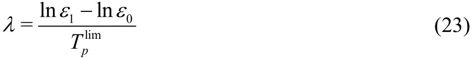
Let us consider a two-dimensional Rayleigh-Bénard convection flow[35,36], as shown in Fig.8. The incompressible fluid between two parallel free surfaces separated by H obtains heat from the bottom boundary due to the constant temperature difference TΔ, from which a reference velocity can be defined by, where is the gravity acceleration and is the thermal expansion coefficient of the fluid, respectively. The corresponding non-dimensional governing equations in the form of stream function with the Boussinesq approximation read[35]:

where θ is the temperature departure from a linear variation background, (x,y) are the horizontal and vertical spatial coordinates, t is the time, ▽2is the Laplace operator defined as ▽4=▽2▽2,

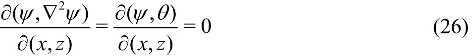
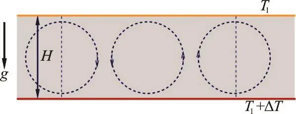
Fig.8 Sch ematic representation of the Rayleigh-Bénard convec- tiveflow.The two-dimensionalincompressiblefluid be- tween two parallel free surfaces

Like Saltzman[35], we express the stream function and temperature departure θ in the double Fourier expansion modes as:

where m, n are the wave numbers in the and z directions, ψm,n(t ) and Θm,n(t)are the amplitudes of

and θ with the wave numbers m, n, respectively. Substituting (27) and (28) into (24), (25) and the boundary conditions (26), we have a set of dynamic system with 2×M×N unknowns ψm,n(t ),Θm,n(t ), where 1 ≤ m ≤ M , 1 ≤ n ≤ M . For details please refer to Lin et al.[20].

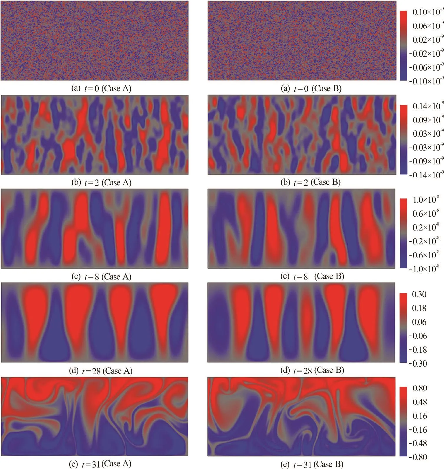
Fig.9 Evolution of the θ (temperature departure fromalinearvariationbackground)field.Theresults are in case of theRayleigh number R a = 107 and the double Fourier expansion modes M = N =127. Case A and case B have different initialmicro-level uncertainty, generated by the same variance of temperature σ T =10-10 and velocity σu=10-9

Without loss of generality, we consider the case of the aspect ratio Γ = L/H =,P r = 6.8 (water)and R a =107, corresponding to a linearly unstable case. Besides, we choose M = N = 127, which is large enough to investigate the laminar-turbulent transition.

Although the Rayleigh-Bénard convection is modeled theoretically as external disturbance isolated,randomness at the microscopic level still exists because of the molecular thermal fluctuation that plays an important role on hydrodynamic instability.For the consideredocases, the fluid is water at the room temperature of 20C, the standard deviations for the temperature and velocity field can be estimated from statistical mechanics[37]as σT=10-10and σu=10-9,respectively.

The inevitable thermal fluctuation is regarded as a Gaussian white noise in mathematics. To gain convergent (reliable) numerical results, the CNS is used to simulate the evolution of the micro-level thermal fluctuation that is much smaller than numerical noises of traditional algorithms in double precision.For given random initial condition, the convergent(reliable) numerical simulations aregained in the interval [0,50] by the CNS usingthe 10th-order Taylor series method, the MP data in the 100-digit precision and time step Δ t =0.005, plus a converg encecheck by an additionalsimulation with even smaller numerical noises (using the 12th-order Taylor series method).

In different cases, the initial temperature and velocity fields are randomly generated as Gaussian white noise, with the same temperature variance σT=10-10and velocity variance σu=10-9, respectively. As shown in Fig.9(a), such tiny difference of the initial condition is negligibly small compared to the background fields at the macroscopic level, and thus the initial status can be physically regarded as the same. As time increases, the filed structures and scales evolve rapidly. The clear large-scale patterns appear even at the very early stage, as shown in Fig.9(b) for t = 2, although the magnitudes are still insensibly small. When t = 8 as shown in Fig.9(c), the largecale structures become more and more distinct.Interestingly, these intermediate structures remain stable in a long interval up to t = 28, as shown in Fig.9(d), while the field energy increases continuously.At a critical point once the field is too energetic to be stable,these large-scale structuresdisintegrate abruptly, leading to the turbulent status, as shown in Fig.9(e) at t = 31. Note that the two flow structures in Fig.9(e) are sharply different, which must originate from the different initial micro-level randomness due to thermal fluctuation. Thus, “the physical limit time of prediction” for the considered Reyleigh-Bénard convection turbulent flow is about 31, say,≈ 3 1,beyond which the considered flow becomes intrinsically random.

It should be emphasized that the CNS can give the reliable numerical results in a long enough time interval with the negligible numerical noises much smaller than the physical uncertainty, while traditional algorithms in double precision fail due to the butterfly effect. Our CNS results suggest that turbulence in the Reyleigh-Bénard convection problem could be selfexcited or “out of nothing”, say, the micro-level thermal fluctuation is the origin of randomness in turbulent flow. It means, even if all external disturbance and man-made uncertainties could be avoided,turbulent flows are always random, forever. Therefore,these CNS results provide us a rigorous theoretical evidence for the “intrinsic randomness” of turbulent flows.

3.4 Discovery of new periodic orbits of three-body prob lem

The famous three-body problem[1]can be traced back to Isaac Newton in1680s. According to Poincaré[1], a three-body system is not integrable in g eneral. Besides, orbits of three-body problem are often chaotic[3], say, sensitive to initialconditions[2,4],although there exist periodic orbits in some special cases.

In the 300 years sincethis “three-body problem”[1]was first recognized,only three families of periodic solutions had been found, until 2013 when Šuvakov and Dmitrašinović[38]made a breakthrough to find 13 new distinct periodic collisionless orbits that belongs to eleven new families of Newtonian planar three-body problem with equal mass and zero angular momentum. Before this, only three families of periodic three-body orbits were found:

(1) The Lagrange-Euler family discovered by Lagrange and Euler in 18th century.

(2) TheBroucke-Hadjidemetriou-Hénon family[39-43].

(3) The Figure-eight family, discovered by Moore[44]in 1993 and rediscovered by Chenciner and Montgomery[45]in 2000.

Hudomal[46]reported 25 families of periodic orbits in 2015, including the 11 families found in Ref.[38].

Currently, Li and Liao[21]considered a planar three-body system governed by the Newton's second law and gravitational law

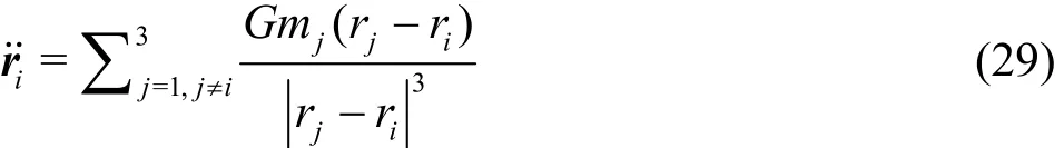
where riand mjare the position vector and mass of the it h body (i = 1,2,3), G is the Newtonian gravity coefficient, and the dot denotes the derivative with respect to the time t, respectively. Like Šuvakov and Dmitrašinović[38], they considered a planar three-body system with zeroangular momentum in the case of G = 1, m1= m2= m3=1,and the initial conditions in case of the isosceles collinear configurations:

specified by the four parameters ( x1,x2,v1,v2). Write y( t) =(r1( t) , r˙1( t)) A periodic solution with the unknown period T0is the root of the equation y( 0)= y( T0). Note that x1= - 1 and x2=0 correspond to the normal case used in Ref.[38] that regards r1(0)=(-1,0) to be fixed. However, unlike Šuvakov and Dmitrašinović[38], we regard1x and2x as variables. So, mathematically speaking, we search for the periodic orbits of this three-body problem using a larger degree of freedom than Šuvakov and Dmitrašinović[38].

First, like Šuvakov and Dmitrašinović[38], we use the grid search method to find candidates of the initial conditions y ( 0)=(x1, x2,v1,v2) for periodic orbits.We choose the initial positions1= 1x -,2=0x and search for the initial conditions of periodic orbits in the two-dimensional plane v1∈ [0 ,1] and v2∈ [ 0,1].We set 1 000 points in each dimension and thus have one million grid points. With these one million different initial conditions, the motion equations (29)subject to the initial conditions (30) are integrated up to the time =100t by means of the ODE solver dop853, which is developed by Hairer et al.[47]and based on an explicit Runge-Kutta's method of order 8(5,3) in double precision with adaptive step size control. If the return proximity function y( 0) - y(T0)is less than 0.1, the corresponding initial conditions and the period T0are regarded as the candidates.

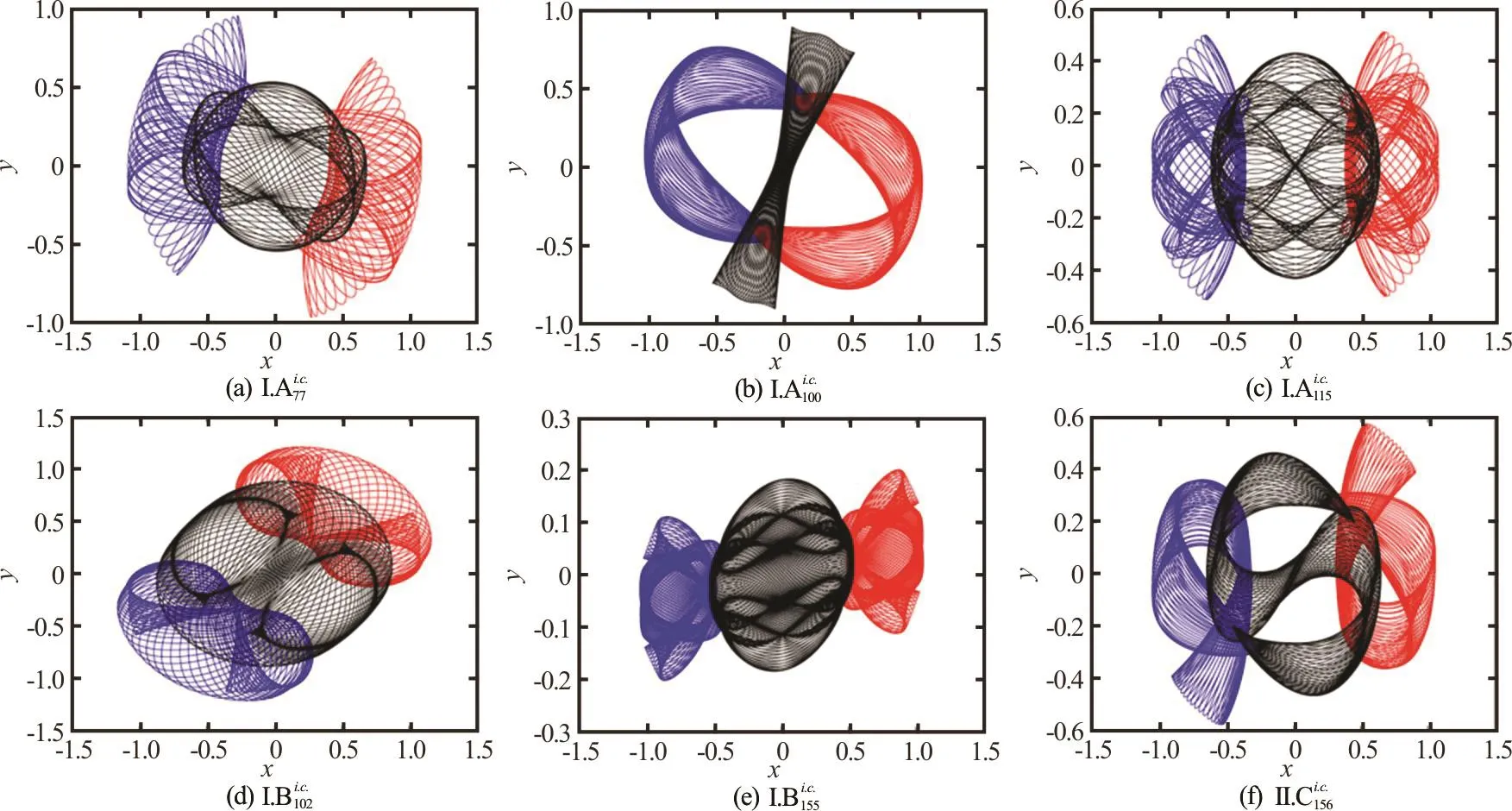
Fig.10 Brief overview of the six newly-found families[21]ofperiodicthree-bodyorbitsincaseofequal mass, zero angularmomentum and initial conditions with isosceles collinear configuration

Secondly, these candidates of the initial conditionsare modified by meansof the Newton-Raphson method[48-50]. At this stage, the motion equations are solvedn[47]merically by means of the sameODE solver dop853. A periodic orbit is found whenthe levelof the return proximity functiony( 0) - y( T0) is less than 10-6. Note that, different from the numerical approach in Ref.[38], not only the initial velocity r˙1( 0 ) = r ˙2( 0)=(v1, v2) but also the initial position r1(0)=(x1, x2)are modified. In other words, our numerical approach also allows r1( 0)=(x1,x2) to deviate from its initial guess (-1 ,0). With such kind of larger degree of freedom, our approach gives 137 families of p eriodic orbits, including the well-knownFigure-eight, the 10 familiesfound byŠuvakov and Dmitrašino, andlots ofcompletely new families that have been never reported. However,one family reported inwas not among these 137 periodic orbits. So, at least one periodic orbit was lost at this stage. This is notsurprising, since three-body problemis notintegrable in and might be rather sensitive to initial conditions, as shown in Sectio ns 3.1and3.2. T herefo re, inste ad of usingtheODEsolverbasedontheRunge-Kutta's method in double precision, Li and Liao[21]used the CNS with the MP data in 100-digit precision and the truncation errors less than 10-70to solve the motion equation (29). In this way, Li and Liao[21]found totally 164 families of periodic orbits in the interval[0,100], say, 27 more orbits are found by means of the CNS than the Runge-Kutta's method in double precision.

It is found by Li and Liao[21]that more periodic orbits can be gained by means of finer search grids.Using 4 000×4 000 search grids for the candidates of initial conditions, they totally gained 695 periodic orbits within 0200t≤≤ by means of the CNS in a similar way. Some new orbits are as shown in Fig.10.For more details, please refer to Li and Liao[21]. The movies of these 695 periodic orbits in the real space can be found via the website:http://numericaltank.sjtu.edu.cn/three-body/three-body.htm

Especially, it should be emphasized that 243 more periodic orbits are found by means of the CNS[21]than the traditional Runge-Kutta's method in double precision[47]. This indicates the great potential of the CNS, since a truly new method should/must bring us something new/different!

4. Concluding remarks

Many nonlinear dynamical systems have the SDIC, which was pointed out first by Poincaré[1]in 1890 and became very famous when Lorenz[2]numerically solved a simple model (i.e., Lorenz equation) by computer in 1963 and gave it a popular name“butterfly-effect”. Due to the butterfly-effect[2], any a tiny difference in initial condition (and also at any time steps) of chaotic dynamic systems exponentially enlarges so that long-term convergent (reliable) simulations of chaos are impossible by means of any traditional algorithms in double precision. These lead to some serious doubts and intense arguments[9,12-14]on the reliability of numerical simulations of chaos.Some researchers[12]even believed that “all chaotic responses are simply numerical noise and have nothing to do with the solutions of differential equations”.

These intense arguments[12,13]should be quieted down by the CNS[15-21], which can give convergent(reliable) chaotic simulations in an arbitrary long (but finite) interval of time with negligible numerical noises much smaller even than micro-level uncertainty of physical quantities under consideration. The CNS is based on the Taylor series method at high enough order of approximation and the MP data with large enough number of digits, plus a convergence check using an additional simulation with even smaller numerical noises. By means of the CNS, numerical noises can be reduced to such a low level that long-term convergent (reliable) simulations of chaos are possible in an arbitrary long (but finite) interval of time, and that even propagation of physical microlevel uncertainty can be investigated precisely. The CNS has been widely applied to solve lots of chaotic dynamic systems, such as the Lorenz equation[18],the three-body problem[17,19,21], the Rayleigh-Bénard convection turbulent flows[20], and so on. For example, the convergent (reliable) chaotic solution of Lorenz equation in a quite long interval of time, i.e., [0,10000], was obtained[18]by means of the CNS, for the first time. This indicates that long-term reliable simulation of chaos is indeed possible in theory.

For the chaotic three-body system[17,19,21], we put forward a new concept “physical limit time of prediction”, denoted by, which gives a timescale for “at most how long a deterministic prediction of chaotic dynamic systems is physically correct”.Using the CNS, it is found that physical micro-level uncertainty of the three-body system might enlarge exponentially and transfer into macroscopic randomness when t ＞. In other words, the physical micro-level uncertainty istheorigin of the macroscopic randomness of the three-body system.Thus, theoretically speaking, it is impossible to give physically correct chaotic trajectories when t ＞.Note that[17,19,21], without any external disturbances,the ten thousand physically same initial conditions of the three-body system lead to completely different orbits after t ＞, together with the symmetry breaking and system disruption. Therefore, the symmetry breaking and system disruption of the three-body system are self-excited, i.e., out of nothing! Besides, the CNS was successfully used[20]to solve turbulent flows governed by the NS equations,as shown in Section 3.3 for the two-dimensional Rayleigh-Bénard convection turbulent flow. With numerical noisesmuch smaller than thermal fluctuation, the CNS provides us, for the first time, a rigorous theoreticalevidence that thethermal fluctuation is the origin of the macroscopic randomness of turbulent flows.

In addition, 243 more periodic orbits of threebody problem were found in Ref.[21] by means of the CNS. This indicates the great potential of the CNS,since a truly new method always must bring us something completely new/different!

In summary, with negligible numerical noises much smaller than all physical quantities in an arbitrary long (but finite) interval of time, the CNS provides us a better numerical tool to more precisely investigate chaotic dynamic systems than traditional algorithms in double precision.

Acknowledgements

I would like to thank all of my co-authors in this research field, Mr. Xiao-min Li, Dr. Zhi-liang Lin, Dr.Li-po Wang in Shanghai Jiao Tong University, and Dr.Peng-fei Wang in Institute of Atmospheric Physics,Chinese Academy of Sciences.

[1] Poincaré J. H. Sur le problème des trois corps et les équations de la dynamique. Divergence des séries de M.Lindstedt [J]. Acta Mathematica, 1890, 13: 1-270.

[2] Lorenz E. N. Deterministic nonperiodic flow [J]. Journal of the Atmospheric Sciences, 1963, 20(2): 130-141.

[3] Li T. Y., Yorke J. A. Period three implies chaos [J].American Mathematical Monnthly, 1975, 82: 985-992.

[4] Lorenz E. N. The essence of chaos [M]. Seattle, USA:University of Washington Press, 1993.

[5] Parker T. S., Chua L. O. Practical numerical algorithms for chaotic systems [M]. New York, USA: Springer-Verlag, 1989.

[6] Smith P. Explaining chaos [M]. Cambridge, UK: Cambridge University Press, 1998.

[7] Sprott J. C. Elegant chaos: Algebraically simple chaotic flows [M]. Singapore: World Scientific, 2010.

[8] Lorenz E. N. Computational periodicity as observed in a simple system [J]. Tellus Series A-Dynamic Meteorology and Oceanography, 2006, 58(5): 549-557.

[9] Teixeira J., Reynolds C. A., Judd K. Time step sensitivity of nonlinear atmospheric models: Numerical convergence,truncation error growth and ensemble design [J]. Journal of the Atmospheric Sciences, 2007, 64(1): 175-189.

[10] Hoover W. G., Hoover C. G. Comparison of very smooth cell-model trajectories using five symplectic and two Runge-Kutta integrators [J]. Computational Methods in Science and Technology, 2015, 21(3): 109-116.

[11] Li J., Zeng Q., Chou J. Computational uncertainty principle in nonlinear ordinary differential equations (I):Numerical results [J]. Science in China Series E, 2000,43(5): 55-74.

[12] Yao L. S., Hughes D. Comment on “computational periodicity as observed in a simple system” by Edward N.Lorenz (2006a) [J]. Tellus Series A-Dynamic Meteorology and Oceanography, 2008, 60(4): 803-805.

[13] Lorenz E. N. Reply to comment by L. S. Yao and D.Hughes [J]. Tellus Series A-Dynamic Meteorology and Oceanography, 2008, 60(4): 806-807.

[14] Yao L. S. Computed chaos or numerical errors [J]. Nonlinear Analysis:Modelling and Control, 2010, 15(1):109-126.

[15] Liao S. On the reliability of computed chaotic solutions of non-linear differential equations[J].TellusSeries A-Dynamic Meteorology and Oceanography, 2009, 61(4):550-564.

[16] Liao S. On the numerical simulation of propagation of micro-level inherent uncertainty for chaotic dynamic systems [J]. Chaos, Solitons and Fractals, 2013, 47(1):1-12.

[17] Liao S. Physical limit of prediction for chaotic motion of three-body problem [J]. Communications of Nonlinear Science and Numerical Simulations, 2014, 19(3): 601-616.

[18] Liao S. J., Wang P. F. On the mathematically reliable long-term simulation of chaotic solutions of Lorenz equation in the interval [0,10000] [J]. Science China Physics,Mechanics and Astronomy, 2014, 57(2): 330-335.

[19] Liao S. J., Li X. M. On the inherent self-excited macroscopic randomness of chaotic three-body systems [J].International Journal of Bifurcationand Chaos, 2015,25(9): 1530023.

[20] Lin Z. L., Wang L. P. and Liao S. J. On the origin of intrinsic randomness of Rayleigh-Benard turbulence [J].Science China Physics Mechanics and Astronomy, 2017,60(1): 14712.

[21] Li X. M., Liao S. J. More than six hundreds new families of Newtonian periodic planar collisionless three-body orbits[J]. Science China Physics Mechanics and Astronomy, DOI: 10.1007/s11432-016-0037-0(accepted).

[22] Oyanarte P. MP-A multiple precision package [J]. Computer Physics Communications, 1990, 59(2): 345-358.

[23] Gibbon A. A program for the automatic integration of differential equations using the method of Taylor series [J].Computer Journal, 1960, 3(5): 108-111.

[24] Barton D., Willers I. M., Zahar R. V. M. The automatic solution of systems of ordinary differential equations by the method of Taylor series [J]. Computer Journal, 1971,14(3): 243-248.

[25] Corliss G., Lowery D. Choosing a step size for Taylor series methods for solving ODEs [J]. Journal of Computational and Applied Mathematics, 1977, 3(4): 251-256.

[26] Corliss G., Chang Y. Solving ordinary differential equations using Taylor series [J]. ACM Transactions Mathatical Software, 1982, 8: 114-144.

[27] Barrio R., Blesa F., Lara M. VSVO formulation of the Taylor method for the numerical solution of ODEs [J].Computers Mathematics with Applications, 2005, 50(1):93-111.

[28] Oberkampf W. L., Roy C. J. Verification and validation in scientific computing [M]. Cambridge, UK: Cambridge University Press, 2010.

[29] Qin S., Liao S. Influence of round-off errors on the reliability of numerical simulations of chaotic dynamic systems[J]. Journal of Applied Nonlinear Dynamics, arXiv:707.04720(accepted).

[30] Li X., Liao S. The influence of numerical noises on statistics computation of chaotic dynamic systems [J]. arXiv Preprint, 2016, arXiv:1609.09354.

[31] Wang P., Li J., Li Q. Computational uncertainty and the application of a high-performance multiple precision scheme to obtaining the correct reference solution of Lorenz equations [J]. Numerical Algorithms, 2012, 59(1):147-159.

[32] Polchinski J. String theory [M]. Cambridge, UK: Cambridge University Press, 1998.

[33] Heisenberg W. Über den anschaulichen inhalt der quantentheoretischen kinematik und mechanic [J]. Zeitschrift für Physik, 1927, 43: 172-198.

[34] de Broglie L. Recherches sur la thèorie des quanta [D].Doctoral Thesis, Paris, France: Université En Coursd'Affectation, 1924.

[35] Saltzman B. Finite amplitude free convection as an initial value problem–I [J]. Journal of the Atmospheric Sciences,1962, 19: 329-34133.

[36] Getling A. V. Rayleigh-Benard convection: Structures and dynamics [M]. Hackensack, USA: World Scientific, 1998.

[37] Khinchin A. I. Mathematical foundations of statistical mechanics [M]. New York, USA: Dover Publications, 1949.

[38] Šuvakov M., Dmitrašinović V. Three classes of Newtonian three-body planar periodic orbits [J]. Physical Review Letters, 2013, 110(11): 114301.

[39] Broucke R. On relative periodic solutions of the planar general three-body problem [J]. Celestial Mechanics, 1975,12(4): 439-462.

[40] Hadjidemetriou J. D. The stability of periodic orbits in the three-body problem [J]. Celestial Mechanics, 1975, 12(3):255-276.

[41] Hadjidemetriou J. D., Christides T. Families of periodic orbits in the planar three-body problem [J]. Celestial mechanics, 1975, 12(2): 175-187.

[42] Hénon M. A family of periodic solutions of the planar three-body problem, and their stability [J]. Celestial mechanics, 1976, 13(3): 267-285.

[43] Hénon M. Stability of interplay motions [J]. Celestial mechanics, 1977, 15(2): 243-261.

[44] Moore C. Braids in classical dynamics [J]. Physical Review Letters, 1993, 70(24): 3675-3679.

[45] Chenciner A., Montgomery R. A remarkable periodic solution of the three-body problem in the case of equal masses[J]. Annals of Mathematics, 2000, 152(3): 881-901.

[46] Hudomal A. New periodic solutions to the three-body problem and gravitational waves [D]. Master Thesis,Belgrade, Serbia: University of Belgrade, 2015.

[47] Hairer E., Nørsett S. P., Wanner G. Solving ordinary differential equations I: Nonstiff problems [M]. Berlin,Germany: Springer-Verlag, 1993.

[48] Farantos S. C. Methods for locating periodic orbits in highly unstable systems [J]. Journal of Molecular Structure: THEOCHEM, 1995, 341(1-3): 91-100.

[49] Lara M., Peláez J. On the numerical continuation of periodic orbits-an intrinsic, 3-dimensional, differential, predictor-corrector algorithm [J]. Astronomy and Astrophysics, 2002, 389(2): 692-701.

[50] Abad A., Barrio R., Dena A. Computing periodic orbits with arbitrary precision [J]. Physical Reiew E, 2011, 84:016701.

July 26, 2017, Revised July 27, 2017)

* Project supported by the National Natural Science Foundation of China (Grant No.1432009)

Biography: shi-jun Liao (1963-), Male, Ph. D., Professor