Development of current-induced scour beneath elevated subsea pipelines

Jun Y. Lee Alexnder L. Forrest b Fuzi A. Hrdjnto Shuhong Chi Remo Cossu Zhi Q. Leong

a National Centre for Maritime Engineering and Hydrodynamics, Australian Maritime College, University of Tasmania, Locked Bag 1395, Launceston Tasmania 7250, Australia

b Department of Civil and Environmental Engineering, University of California -Davis, Davis, CA 95616, United States

c School of Civil Engineering, University of Queensland, St Lucia Queensland 4072, Australia

Abstract When scour occurs beneath a subsea pipeline and develops to a certain extent, the pipeline may experience vortex-induced vibrations,through which there can be a potential accumulation of fatigue damage. However, when a pipeline is laid on an uneven seabed, certain sections may have an elevation with respect to the far-field seabed, e o , at which the development of scour would vary. This work focused on predicting the development of the scour depth beneath subsea pipelines with an elevation under steady flow conditions. A range of pipe elevation-to-diameter ratios (i.e. 0 ≤ e o / D ≤ 0.5) have been considered for laboratory experiments conducted in a sediment flume. The corresponding equilibrium scour depths and scour time scales were obtained; experimental data from published literature have been collected and added to the present study to produce a more complete analysis database. The correlation between existing empirical equations for predicting the time scale and the experimental data was assessed, resulting in a new set of constants. A new manner of converting the scour time scale into a non-dimensional form was found to aid the empirical equations in attaining a better correlation to the experimental data.Subsequently, a new empirical equation has also been proposed in this work, which accounts for the influence of e o / D on the non-dimensional scour time scale. It was found to have the best overall correlation with the experimental data. Finally, full-scale predictions of the seabed gaps and time scales were made for the Tasmanian Gas Pipeline (TGP).

Keywords: Scour time scale; Equilibrium scour depth; Subsea pipelines; Pipe elevation; Steady currents.

1.Introduction

1.1. Background

Pipeline networks across the globe which stretch up to tens of thousands of kilometres along the seabed are said to be the lifeline of the oil industry [1] . Scour can occur around the pipeline due to excessive fluid forces. The erosion of sediment underneath the pipe may lead to the occurrence of vortex-induced vibrations, or having excessive bending moments, which may compromise the structural integrity of the pipe. However, a pipeline may be found at a certain distance from the seabed [1] (e.g. Fig. 1 ), and pipeline free-spans can be permanent [2] . If the span length, hydrodynamic loads and pipe characteristics are such that unacceptable fatigue damage can develop or, even worse, the critical bending moment is exceeded, intervention works to mitigate these occurrences shall be undertaken. However, rectification works, such as rock dumping, are expensive (e.g. approximately $US1.2 million per kilometre [3] ). Furthermore, for a smaller pipe elevation,eo, a larger amplification of the seabed shear stress beneath the pipe can be expected, and hence a deeper scour hole [4] .

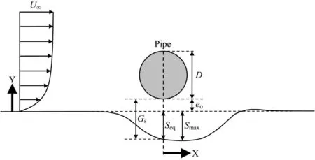
Fig. 1. Two-dimensional sketch of scour beneath a suspended section of a pipeline with an elevation with respect to the far-field seabed, e o ; the seabed gap,G s , is defined as the summation of the pipe elevation and the scour depth directly beneath the pipe.

Table 1 Comparison of equations for predicting the equilibrium scour depth, listed in chronological order.

It is of technical interest to predict the development of the scour hole beneath the pipeline, or more specifically, the time required to reach a significant scour depth, where for example, storm events may not last as long as the period required for the scour hole to reach an equilibrium state [5] . Although the influence ofeo/Dhad been considered for predicting the maximum seabed shear stress and equilibrium scour depth beneath the pipe, it had not been considered in terms of predicting the scour time scale. In this work, we focus on predicting the time scale of two-dimensional scour occurring beneath a pipeline with an elevation under steady currents.

1.2. Literature review

1.2.1.Equilibriumscourdepth

With regards to predicting the equilibrium scour depth,Seq, for steady currents, several equations have been proposed over the years ( Table 1 ). Kjeldsen et al. [6] formulated an equation via flume experiments, whereUo2/2gis the velocity head. However, this equation appears to have been developed for bottom-seated pipelines (i.e.eo/D= 0), and the influence of the sediment properties has not been considered. Even though not fully non-dimensionalized, Bijker and Leeuwestein [7] modified the aforementioned equation based on more experimental data, and quantified the influence of the mean sediment grain size,d50, which seems to be relatively small.

Ibrahim and Nalluri [8] extended this work by proposing two non-dimensional equations: one for the clear-water condition; and, one for the live-bed condition. In these equations,Uois the undisturbed mean flow velocity,Ucis the critical velocity for sediment entrainment, andhis the water depth.The clear-water condition refers to the scenario whereby the upstream seabed shear stress is lower than the critical value for sediment transport to occur far away from the pipe (i.e.θ∞＜ θcr); conversely, for the live-bed condition, the upstream seabed shear stress is greater than the critical value(i.e. θ∞＞ θcr). However, there are contradicting exponents in the two equations proposed by Ibrahim and Nalluri [8] .Furthermore, havingSeq/D＞ 0 whenUo= 0 m/s may not be practically sound.

Subsequently, Fredsøe et al. [9] claimed that the dimensionless equilibrium scour depth,Seq/D, due to steady currents is 0.6 for all practical purposes. Moncada-M and Aguirre-Pe[10] , who investigated scour beneath pipelines in river crossings, later showed thatSeq/Dis significantly influenced by the Froude number andeo/D. This may be the case due to the fact that the experiments mostly involved a water depth ratio,h/D, of less than 4. Nevertheless, this is the first time the effects ofeo/Dhave been included in an equation for the prediction ofSeq/D.

Sumer and Fredsøe [1] also reported that the equilibrium scour depth can be significantly influenced byeo/D; however,eo/Dis the only term which has been included in the equation, with the notion that it is only applicable for the live-bed condition. More recently, Lee et al. [4] proposed an equation that included the upstream dimensionless seabed shear stress,θ∞, and is applicable for both clear-water and live-bed conditions. In addition, the influence of the Reynolds number had been quantified, though it is small. Nonetheless, this equation, which is presented in Table 1 appears to be the most comprehensive equation for predictingSeq/Dto date.

On a separate note, Chao and Hennessy [11] proposed an iterative method to compute the scour depth based on potential flow theory. However, this method only provides a prediction of the order of magnitude of the scour depth. The limitation in the accuracy can be attributed to the negligence of fluid viscosity, and consequently, the absence of flow separation occurring downstream of the pipe [12] . Chiew [12] and Dey and Singh [13] proposed improved, but more complicated iterative methods to predict the equilibrium scour depth, whereby the iteration process involves estimating a scour depth that would result in a seabed shear stress beneath the pipe which is equal to the critical shear stress for the sediment. Thus, it is assumed that the scour hole will not develop any further as the shear stress is equal to or below the critical value. However, this might only be valid for the clear-water condition;otherwise, the upstream seabed shear stress would exceed the critical value for the live-bed condition. Therefore, this work referred to the closed-form equation from Lee et al. [4] in terms of predictingSeq/D.

1.2.2.Scourtimescale

The following equation was commonly used to describe the development of the scour depth beneath a pipe [9] :

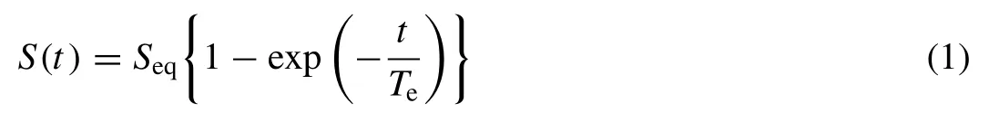
whereS(t) is the change in the absolute value of the scour depth beneath the pipe with time;Seqis the equilibrium scour depth;tis time in seconds; and,Tehas been defined as the time required for substantial scour to develop. A nondimensional form of the time scale,Te∗, was also proposed in [9] :

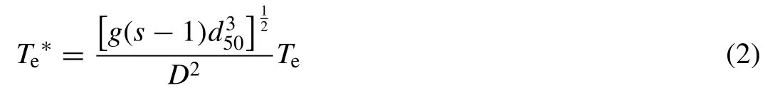
wheregis gravitational acceleration;sis the specific gravity of the sediment;d50is the mean sediment grain size; and,Dis the external pipe diameter. Using Eq. (1) and Eq. (2) as the foundation, several empirical equations have been developed to predict the non-dimensional scour time scale ( Table 2 ).Fredsøe et al. [9] analysed experimental data from [6 , 14] ,and reported that the time scale mainly decreased with the upstream dimensionless seabed shear stress, θ∞, suggesting that the time taken for the scour depth to reach a considerable depth would reduce as the upstream seabed shear stress increased. Hence, Fredsøe et al. [9] proposed an equation where the non-dimensional time scale,Te∗, is inversely proportional

to θ∞ .

Dogan and Arisoy [15] resumed Fredsøe et al.'s [9] work by quantifying the effects of the Keulegan-Carpenter (KC)number on the scour time scale. Two additional equations have been proposed, which are presented in Table 2 , as they resulted in a better correlation with experimental data, as compared to the equation with just the θ∞term; however, different coefficients have been suggested for the clear-water and live-bed cases. The clear-water case refers to a condition in which θ∞is less than the critical shear stress for the sediment, whilst conversely, the live-bed case refers to a condition in which θ∞exceeds the critical shear stress. Subsequently,two additional equations are proposed, wherein theKCnumber is replaced with the modified Ursell parameter,Urp[16] .However, the associated correlation coefficient is lower than that for the equations with theKCnumber. In addition, the influence of the pipe elevation,eo, had not been considered.

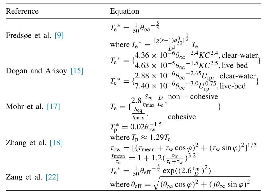
Table 2 Comparison of equations for predicting the scour time scale, listed in chronological order.

Mohr et al. [17] studied the effect of the type of sediment on the scour time scale under steady flow conditions.The equation from Fredsøe et al. [9] was found to perform well in terms of predicting the time scale for non-cohesive sediment (e.g. coarse sand); however, it under-predicted the time scale for cohesive sediment (e.g. very fine sand with a high clay content). Therefore, two new equations have been proposed for predicting the dimensional scour time scale: one for non-cohesive sediment, whereby the transport of sediment is mainly in the form of bed load; and, the other for cohesive sediment, which is largely transported via suspension. With reference to Table 2 , ηmaxis the maximum apparent erosion rate,Dis the pipe diameter, andLcis the stream wise length of the sediment container. These equations have been derived based on a control volume analysis. The erosion rate is calculated based on the upstream seabed shear stress and a critical shear stress, which is determined from erosion testing conducted in Mohr et al. [17] . However, there are potential limitations as physical erosion testing would be required to obtain ηmax. In addition, the applicability to field conditions is unclear asLcwould be very large.

Zhang et al. [18] conducted experiments for the live-bed condition, involving steady currents and waves, and reported that a higher correlation with the experimental data was at-tained by replacing θ∞with θcw, where θcwis a function of the upstream shear stress due to steady currents, τc, and the upstream shear stress due to waves, τw, and ϕ is the flow incidence angle. This meant that, for the case of steady currents, θcwwould be equivalent to the dimensionless seabed shear stress due to currents, which is defined as θ∞in this paper. The equation in Zhang et al. [18] is also developed based on experiments conducted with bottom-seated pipes(i.e.eo/D= 0), and with the flow being perpendicular to the pipe for all cases; nonetheless, it is worth mentioning that Zhang et al. [18] found the following equation from Whitehouse [19] to be capable of attaining a very high correlation coefficient, in terms of the development of the scour hole:

whereCpis a constant for which the value is determined via a least-square fit, and ifCp= 1, then Eq. (3) would be equivalent to Eq. (1) . Eq. (3) is later used in this work to estimate the dimensional scour time scale,Tp, where the best fit ofTpandCpare found for each test case.

There have been previous work that focused on the influence of the vertical position of the pipe with respect to the far-field seabed. Numerical simulations [20 , 21] have been performed, to investigate the effects of having a pipe sagging into a scour hole, which was initially generated with a stationary pipe. A lower sagging rate was found to increase the final scour depth, while with high sagging speeds, the pipe may reach the bottom of the seabed before any substantial scour can take place. More recently, Zang et al. [22] experimentally investigated the influence of the partial embedment depth,em, and the angle of the incident flow, ϕ, on the scour time scale, for the live-bed condition. The equation shown in Table 2 included an effective dimensionless shear stress, θeff,and the embedment ratio,em/D, where θeffwould be equivalent to θ∞for the case of having the flow perpendicular to the pipeline. This differed from the scenario in which a pipe is sagging into a pre-existing scour hole, as the pipe is partially buried at the beginning. However, it would not be appropriate to apply the equation from Zang et al. [22] to the prediction of the scour time scale beneath a pipe with an elevation,eo.Therefore, this work investigated the influence ofeo/Don the scour time scale, with a particular focus on the clear-water condition, which had not been considered in previous studies.In addition, the Reynolds number effect is also considered,since it had been reported to influence the equilibrium scour depth [23] .

1.3. Outline

Based on the literature review, the influence of the pipe elevation with respect to the far-field seabed had been quantified for the equilibrium scour depth, but not the scour time scale. We conducted experiments in a sediment flume, through which the development of the scour depth beneath an elevated pipe under steady currents was investigated. The experimental results from this study and published literature were used to develop new empirical equations, which were then employed to make predictions for a full-scale pipeline. The methods undertaken to obtain the results, as well as the presentation and discussion of the results are presented in subsequent sections of this paper.

2.Methods

The equilibrium scour depths and scour time scales were obtained for a range of pipe elevation ratios under steady currents via sediment flume experiments. Eq. (3) was fitted to the experimental measurements to obtain the dimensional scour time scale,Tp, and a unique constant,Cp, for every test case. Subsequently, experimental data from published literature were compiled, and the scour time scale was converted to a non-dimensional form. Existing and newly developed empirical equations were used to predict the dimensionless equilibrium scour depths and scour time scales, where the predictions were compared with experimental measurements.Finally, full-scale predictions of the equilibrium scour depth and time scale were also made for a natural gas pipeline (i.e.Tasmanian Gas Pipeline), which were compared against field measurements of the seabed gaps in [24] .

2.1. Sediment flume experiments

Experiments were conducted in a sediment flume with a test section of 6.82 m in length, 0.46 m in width, and 0.61 m in depth at the University of California, Davis. A sketch of a cross-section of the sediment flume, which has an open top section, is shown in Fig. 2 . A steady flow would enter the flume from a tank, which was located at a fixed height on the roof of the building via gravity, whereby the flow rate and water depth were controlled by the opening and the height of the tailgate. A 2.62 m long and 0.15 m deep sandbox, which was filled with Cemex #0/30 sand with a mean grain size,d50, of approximately 0.52 mm, was supported by 6 mm-thick Perspex which were attached to the bottom and sides of the flume. A smooth PVC pipe with an external diameter,D, of 48 mm and thickness of 2 mm was rigidly positioned at various elevations above the sand bed. The pipe was positioned sufficiently far downstream from the inlet to ensure that the flow is fully developed when it encountered the pipe. The development of the scour depth directly beneath the vertical centreline of the pipe was measured using a transparent 300 mm ruler with an accuracy of ±1 mm. A Panasonic Lumix DMC-GF1 camera was set to capture the scour process every second, where the accuracy of the scour time scale measurement was estimated to be ±1 s; however, the scour depths have also been recorded manually for each test case. Similar to [17] , the scour depth was observed to be slightly deeper at the side walls of the flume, and thus the scour depths at the middle of the pipe were recorded instead, to remove this boundary effect.

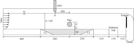
Fig. 2. Sketch of the sediment flume experimental setup, where the external pipe diameter, D , is 48 mm.

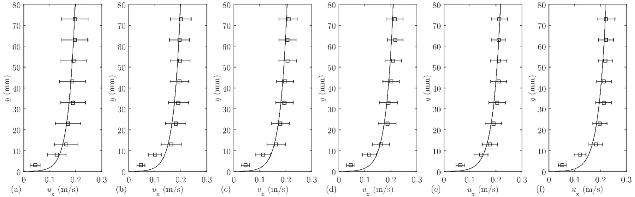
Fig. 3. Stream-wise flow velocity profiles measured at: (a) 2.8 m upstream from the pipe; (b) 2.3 m from the pipe; (c) 1.8 m from the pipe; (d) 1.4 m from the pipe; (e) 1.0 m from the pipe; and, (f) 10 D from the pipe. The error bars represent the standard deviation, and the lines were plotted using Eq. (4) .

The flow velocities were measured using a Nortek Vector Current Meter, which is an Acoustic Doppler Velocimeter(ADV) that relies on the Doppler effect, at a rate of 32 Hz;further details on ADVs can be found in [25] . The accuracy for the water velocity measurements was reported to be ±0.5% of the measured value, whilst the temperature sensor had an accuracy of ± 0.1 °C [26] . As tap water was used with a mean water temperature of approximately 22 °C, hence the water density, ρ, and kinematic viscosity, ν, were taken to be 997.7735 kg/m3and 9.5653 ×10-7m2/s, respectively [27] .

With reference to Fig. 2 , the ADV was placed 10Dupstream from the pipe to measure the flow velocities at various heights (i.e. 10 mm intervals) for every test case. The mean stream-wise flow velocities at each vertical position were attained by averaging the velocities, which were recorded for over one minute. Fig. 3 shows the flow velocities that were measured at different distances upstream from the pipe for one case, wherein the lines were plotted using [28] :

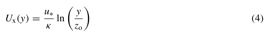
WhereUxis the mean stream-wise flow velocity;u∗is the friction velocity; the von Kármán constant, κ = 0.4 [28, 29] ;yis the elevation from the sand bed; and,zois the bed roughness height. The bed roughness height was estimated via a combination of the following assumptions: (1) where the flow is hydrodynamically rough [28] , and hencezo=ks/30, whereksis the Nikuradse roughness; subsequently, ( 2 )ks= 2.5d50[29 , 30] , whered50is the mean sediment grain size. Thus,the bed roughness height was estimated based on the equivalent mean sediment grain size, wherebyzo=d50/12. There are discrepancies between the calculated and measured velocities close to the sand bed, because Eq. (4) was reported to be valid from a few centimetres above the bed [28] .

Overall, there seem to be small differences in the boundary layer thickness and velocities for different locations, especially at the locations which are close to the pipe. For example, aty= 73 mm from the sand bed, the difference between the mean velocity at 10Dfrom the pipe and that at 1 m from the pipe is approximately 3.4%; while aty= 43 mm from the sand bed, the difference between the mean velocity at 10Dfrom the pipe and that at 1 m from the pipe is approximately 1.5%. In addition, when the velocities were measured at locations that were closer to the pipe, the standard deviations were seen to decrease and approach a relatively constant value.

The test conditions are listed in Table 3 . Various pipe elevation ratios,eo/D, were investigated under the clear-water condition, with a particular focus on relatively small elevations (i.e.eo/D≤0.3), where the capacity for scour to occur was expected to be higher [24] . The experiments were primarily conducted under the clear-water condition, where the upstream dimensionless bed shear stress is below the critical value, due to the lack of published experimental data for the clear-water condition, and to avoid having the effects of scour developing from the upstream edge of the sandbox on the development of the scour hole directly underneath the pipe. The corresponding pipe Reynolds number may be small due to the low flow velocities under the clear-water condition. However,a previous study found the influence of the Reynolds number on the maximum dimensionless bed shear stress beneath the pipe and the equilibrium scour depth to be small [4] . The measured water depths listed in Table 3 may not appear to be precisely constant; however, the standard deviation was only less than 2% of the mean value of approximately 6.04. Larger water depths were not investigated due to physical limitations of the flume. It is also worth mentioning that no small initial hole was made beneath the pipe, whereby the scour process was left to be initiated naturally for every test case.

Table 3 Sediment flume experimental test conditions; d 50 = 0.52 mm; θcr = 0.030.

2.2. Time scale formulation

The main parameters of interest with regards to the sediment flume experiments were the equilibrium scour depth and the scour time scale under steady currents. Upon obtaining the experimental data, published data [14 , 17] have also been compiled, with the aim of developing an equation for predicting the scour time scale. Firstly, Eq. (3) was fitted to every test case, as well as experimental data compiled from published literature [14 , 17] , to estimate the scour time scale,Tp[18 , 19] . The values ofTpandCpwere estimated via:

·having their value initially set to one;

·calculating the difference between the measured values ofSobtained via the experiments andSestimated using Eq. (3) ;

·using unconstrained nonlinear optimization [31] (i.e. via thefminsearchscalar objective function in MATLAB) to iteratively compute the values that would result in the small-est squared difference, thus resembling the ‘least squares'approach; and,

·assessing the corresponding squared correlation coefficient,R2, which was calculated via [18] :

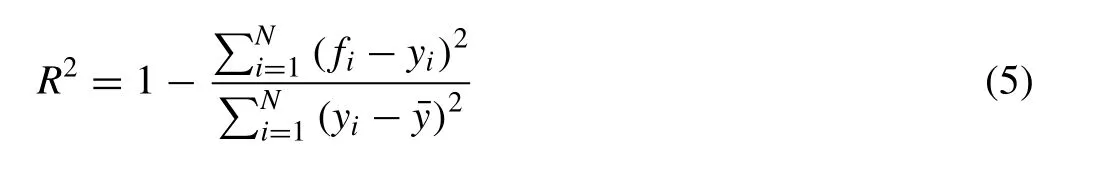
wherefiis the value ofSpredicted via Eq. (3) ;yiis the measured value ofSobtained from the experiments; and, ¯yis the mean of the measured values ofSwhich were obtained via experiments. A unique value ofCpwas attained for each test case in order to achieve highR2values overall, and thus Eq. (3) was able to produce a more accurate estimate of the scour time scale as compared to Eq. (1) from [9] , which is the equivalent of Eq. (3) withCp= 1.

Subsequently, the estimated scour time scale,Tp, was converted into a non-dimensional form,Tp∗, with reference to Eq. (2) which was originally derived in [9] :

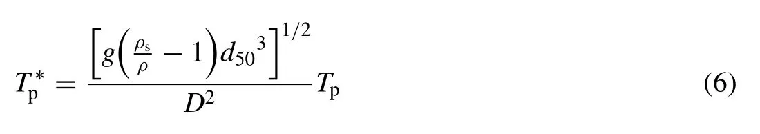
where ρsis sediment density and ρ is fluid density. Finally,several equations were compared for predicting the dimensionless scour time scale, where their correlation to the experimental data were quantified. With reference to the equations proposed in [9 , 18] , a general form was used as follows:

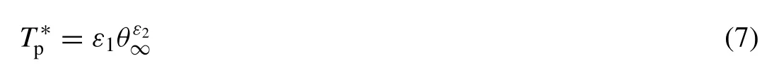
where the values of the constants, ε1and ε2, were computed using the aforementioned optimisation process. A general form of the equation proposed by [22] was also included in this comparison:

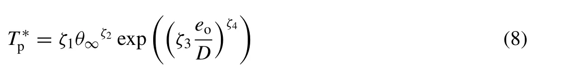
where the values of the constants, ζ1, ζ2, ζ3, and ζ4, were computed using the same optimization process.eo/Dis defined as the dimensionless pipe elevation in this work, even though Eq. (8) was initially proposed in [22] for predicting the scour time scale for pipelines with a partial embedment.Hence, it was thought that updated constants were required.

As it was later found that Eqs. (7) and (8) did not yield a high squared correlation coefficient,R2, a new relationship proposed in this work, Eq. (9) , was later used to normalize the scour time scale, instead of using Eq. (6) [9] :

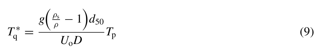
whereUois the depth-averaged current velocity. Eq. (9) was found to enable a better correlation with the experimental data to be attained, in terms of developing an equation for predicting the dimensionless scour time scale. Therefore,Eqs. (7) and (8) were modified into the following equations(i.e. fromto), whilst maintaining the same general forms as before:

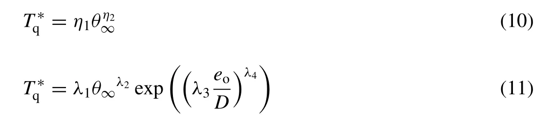
In addition to the aforementioned equations with updated constants, the following equation is proposed in an effort to attain the highest possible correlation to the experimental data:

The Reynolds number, albeit posing a small influence on the maximum bed shear stress beneath the pipe and the equilibrium scour depth [4] , was an interesting parameter to investigate nonetheless. Thus, quantifying the influence ofReon the scour time scale was also done in this work. Theh/Dterm was included in Eq. (12) because it had previously been reported to have an influence on the scour time scale [32] .In this work, Eq. (12) was formulated in such a manner to ensure that:

· wheneo/D= 0, cosh( Ψ5eo/D) = 1, and thusdoes not tend towards zero or infinity;

· whenh/Dtends towards infinity, 1 -sech( Ψ3h/D+ Ψ4)does not tend towards zero or infinity, and thusdoes not tend towards zero or infinity.

Further discussions regarding the formulation of Eq. (12) are presented in subsequent sections of this paper.

3.Results

Experiments were conducted in a sediment flume facility to investigate the development of scour underneath a pipeline with an elevation with respect to the far-field seabed. This work particularly focused on the clear-water condition, for which the upstream shear stress is below the critical shear stress, as there seemed to be a lack of clear-water data in published literature, but live-bed data from multiple sources have been included nonetheless.

3.1. Equilibrium scour depth

Fig. 4 depicts the relationship between the upstream dimensionless bed shear stress, θ∞, and the equilibrium scour depth beneath the pipe,Seq/D, where experimental data from[10 , 14 , 17] were compiled and plotted with results from the present study. The present experimental results was observed to agree with the findings in [14] , where bySeq/Dincreased rapidly with θ∞for the clear-water condition. However, the live-bed data suggest that the relationship betweenSeq/Dand θ∞became less significant at high values of θ∞. With reference to Fig. 5 ,Seq/Dwas seen to increase with the Reynolds number,Re, in the present study (i.e. mostly clear-water).However, the overall relationship betweenSeq/DandRe,which includes both clear-water and live-bed data, was observed to be weak when the data from other sources were put into perspective. In terms of the water depth or blockage ratio,h/D, the results in Fig. 6 suggest that deeper scour depths can be expected at very shallow water depths; however,the influence ofh/DonSeq/Dappeared to be diminishing ash/Dincreased. Fig. 7 suggests that the pipe elevation ratio,eo/D, was seen to have a strong influence onSeq/D, wherebySeq/Dwas observed to decrease with an increase ineo/Dfor both clear-water and live-bed conditions, and thus reinforcing the importance of investigating the effects ofeo/D. This relationship can also be seen in Table 4 for the clear-water condition, wherein for the same depth-averaged current velocity, the resultingSeq/Dgenerally decreased with an increase ineo /D.

Fig. 4. Compilation of experimental data [10 , 14 , 17] showing the correlation between the equilibrium scour depth, S eq / D , and the upstream dimensionless seabed shear stress, θ∞ .

Fig. 5. Compilation of experimental data [10 , 14 , 17] showing the correlation between the equilibrium scour depth, S eq / D , and the Reynolds number, Re .

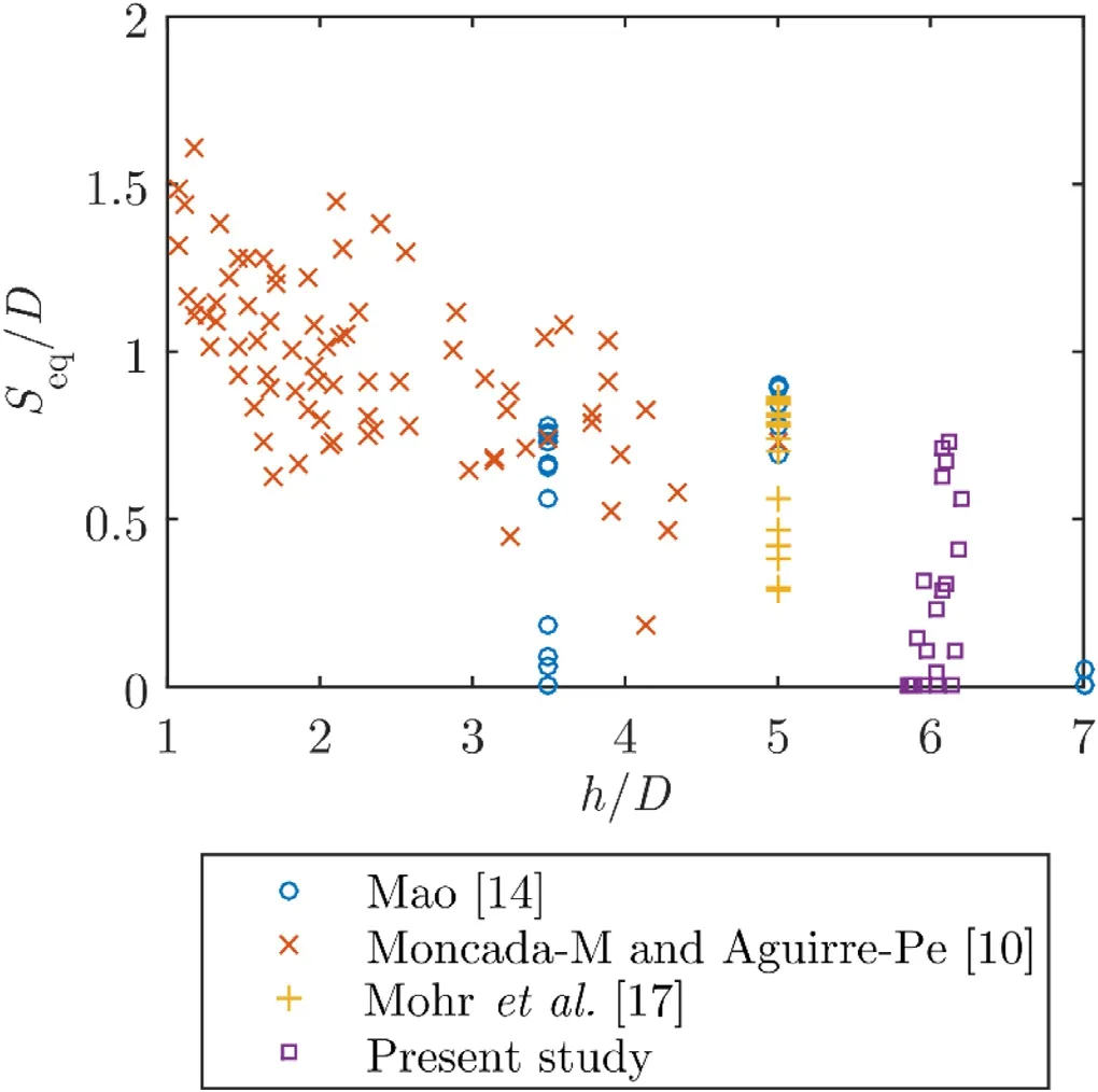
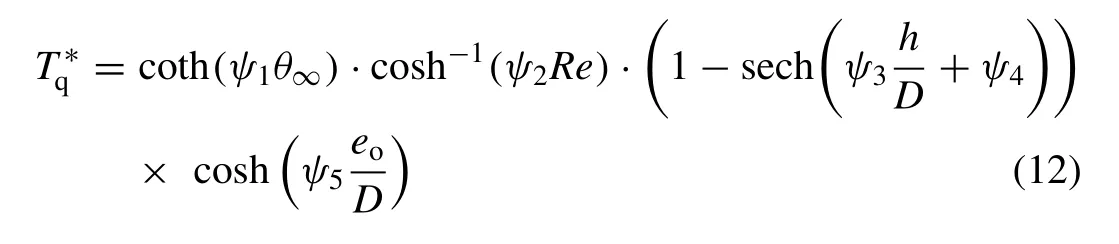
Fig. 6. Compilation of experimental data [10 , 14 , 17] showing the correlation between the equilibrium scour depth, S eq / D , and the water depth or blockage ratio, h / D .

Fig. 7. Compilation of experimental data [10 , 14 , 17] showing the correlation between the equilibrium scour depth, S eq / D , and the pipe elevation ratio,e o / D .

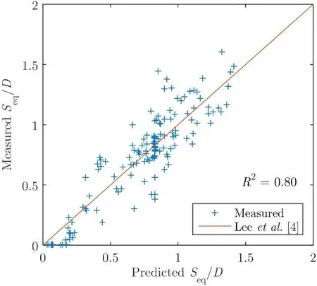
Fig. 8. Correlation between Eq. (13) [4] and the compiled experimental data.

Fig. 8 portrays the correlation between the measured valuesSeq/D, which included results from the present study ( Table 4 ) and from published literature [10 , 14 , 17] , and the values predicted using the following equation [4] :

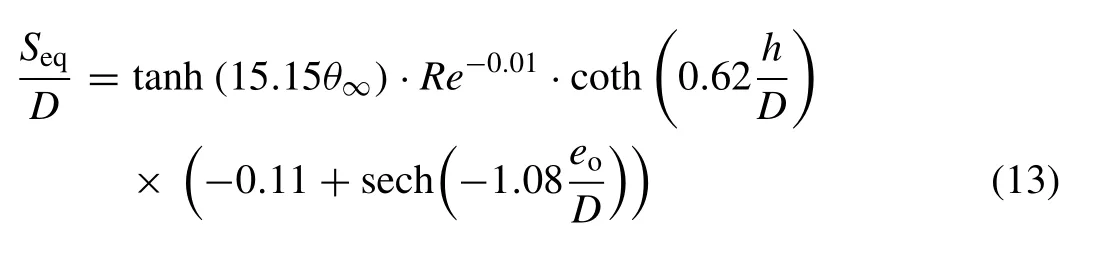
where a very good agreement was observed (i.e.R2= 0.80).In addition, the aforementioned observations based on the experimental data were also consistent with the formulation of Eq. (13) : (1) the initial rapid increase ofSeq/Dwith θ∞,followed by a weak trend at higher values of θ∞( Fig. 4 ),resembled a hyperbolic tangent curve; (2) the overall weak relationship betweenSeq/DandRe( Fig. 5 ) can serve as an explanation for the small coefficient for theReterm; (3) the diminishing influence ofh/DonSeq/D( Fig. 6 ) resembled a hyperbolic cotangent curve; and, (4) inverse relationship betweenSeq/Dandeo/D( Fig. 7 ) resembled a hyperbolic secant curve.

Table 4 included a dimensionless seabed shear stress ratio,θmax/ θcr, which was used to predict the initiation of scour beneath the pipe. The maximum dimensionless seabed shear stress beneath the pipe, θmax, was calculated using [4] :

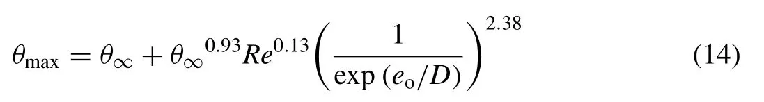
which was normalised by the critical dimensionless shear stress, θcr, at which significant sediment transport beneath the pipe would occur. Eq. (14) was proposed in Lee et al. [4] to estimate the likelihood of scour to occur and progress towards an equilibrium state. This equation was developed based on numerical data, where a large parametric study was performed to compute the maximum seabed shear stress beneath a pipe under various conditions. θcrwas estimated using [28] :

Table 4 Experimental results.

whereD∗, which is the dimensionless form of the sediment grain size, was calculated using [28] :

When θmax/ θcr＞ 1, scour can be expected to occur beneath the pipe. With reference to Table 4 , the dimensionless seabed shear stress ratio, θmax/ θcr, was seen to correlate well with the equilibrium scour depth beneath the pipe,Seq/D, whereby a scour depth was generally not observed when θmax/ θcr＜ 1.The exception would be test number 18, for which θmax/ θcrwas approximately 1.2, whilst no scour was observed. This exception could be attributed to the reliability of Eqs. (14) and(15) . Nonetheless, the adoption of the θmax/ θcrratio to predict the occurrence of scour was seen to be relatively accurate,especially for smalleo/Dratios.

3.2. Time scale

Fig. 9 presents the development of the scour depths beneath the pipe for the test cases wherein scour have occurred underneath the pipe. The best fit curves were plotted using Eq. (3) , for which the associated values, such as the estimated dimensional scour time scale,Tp, the constant,Cp, and the corresponding squared correlation coefficients,R2, are listed in Table 4 . In this work, the method of calculating the area under the curve in order to estimate the scour time scale,which was used in previous studies [9 , 18] , was not adopted for the sake of consistency, where only Eq. (3) was used to estimate the scour time scale. The lowestR2of 0.96 ( Table 4 ) suggests that Eq. (3) is able to produce a very good correlation with the experimental data, which would not have been achievable with the equation from [9] wherebyCp= 1.Higher scour depths were observed for higher current velocities. However, the scour time scale did not necessarily increase with the increase in current velocity. An occasional decrease in the scour time scale was observed, which was also reported in [9] . There seemed to be a clearer influence ofeo/D, whereSeq/Ddecreased with an increase ineo/D, andTpincreased with an increase ineo/D.

In order to better understand the relationship between the manipulated variables and the scour time scale, the time scale was non-dimensionalized. In Fig. 10 , the non-dimensional time scale,, was calculated using Eq. (6) , which is proposed in [9] , whilstwas calculated using Eq. (9) , which is proposed in this work. There does not seem to be a clear relationship between the dimensional time scale,Tp, and the upstream dimensionless bed shear stress, θ∞, as shown in Fig. 10 a. However, an overall downward trend can be observed in both Fig. 10 b and c, wherein the non-dimensional scour time scale was seen to decrease with an increase in θ∞.This overall downward trend is consistent with the findings in previous studies (e.g. [9, 18] ).

Fig. 11 depicts the influence of the Reynolds number on the scour time scale. Similar to the case for θ∞, a clear relationship betweenTpandRewas not observed in Fig. 11 a;however, both Fig. 11 b and c portray a slight downward trend. Although the gradients were not as steep as that seen in Fig. 10 b and c, it is still evident thatReposed an influence on the scour time scale, and thus theReterm was included in Eq. (12) for predicting the non-dimensional scour time scale,which has not been considered in previous studies.

Fig. 9. Development of the absolute scour depth ratio, S / D , over time, where the best fit curves were plotted using Eq. (3) .

Fig. 12 shows the effect of the water depth ratio,h/D, on the scour time scale. There seemed to be an increase in the non-dimensional time scale with an increase inh/D, which agreed with the numerical results in [32] . Due to physical limitations, it was not possible to consider higher water depths.

Fig. 13 shows the effect ofeo/Don the scour time scale,where the time scale appeared to be increasing with an increase ineo/Dfrom an overall perspective, in terms of the dimensional and non-dimensional time scales, despite the fact thatSeq/Ddecreased with an increase ineo/D.

Fig. 10. Correlation between the upstream dimensionless seabed shear stress,θ∞ , and: (a) the dimensional scour time scale, T p , which was estimated using Eq. (3) [18 , 19] ; (b) the non-dimensional scour time scale, T p ∗, which was calculated using Eq. (6) [9] ; and, (c) a new non-dimensional form of the scour time scale, T q ∗, which was calculated using Eq. (9) .

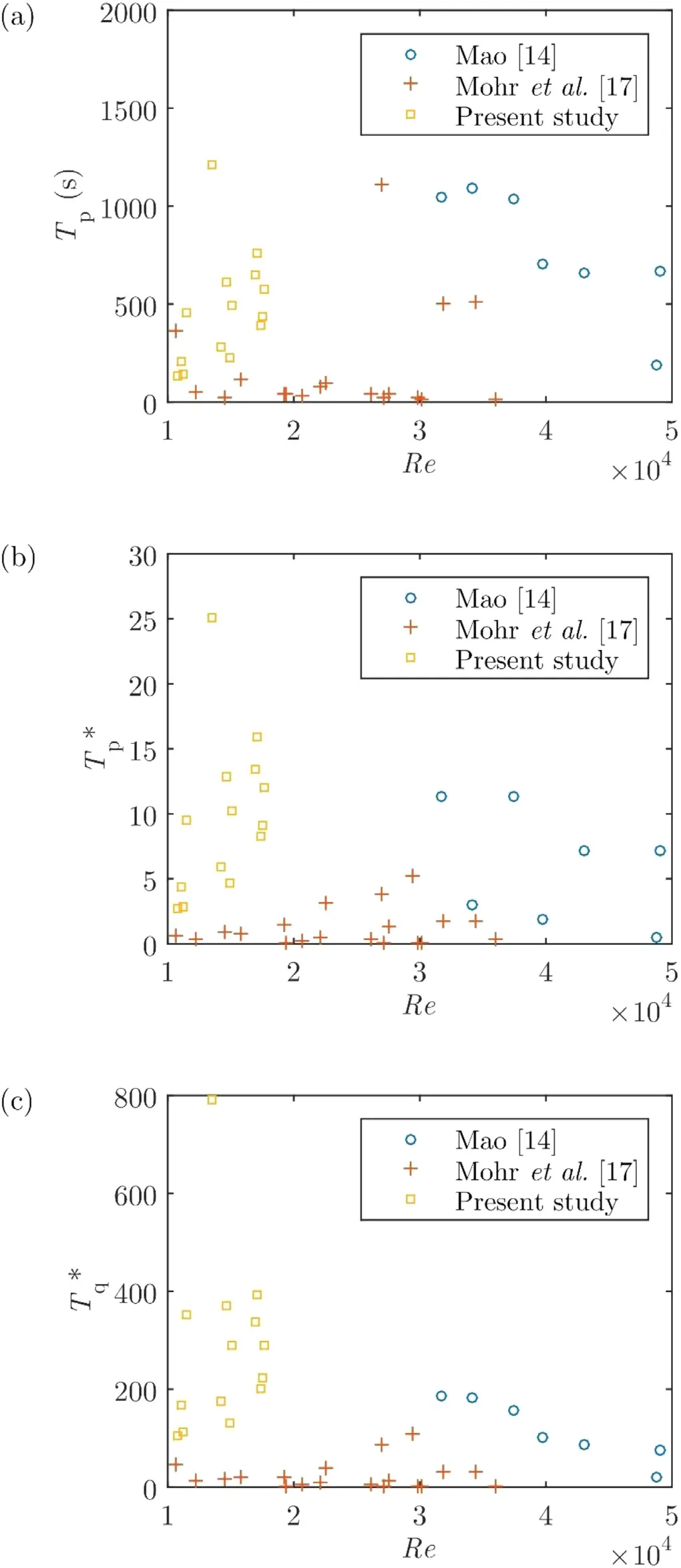
Fig. 11. Correlation between the Reynolds number, Re , and: (a) the dimensional scour time scale, T p , which was estimated using Eq. (3) [18 , 19] ;(b) the non-dimensional scour time scale, T p ∗, which was calculated using Eq. (6) [9] ; and, (c) a new non-dimensional form of the scour time scale,T q ∗, which was calculated using ( 9 ).

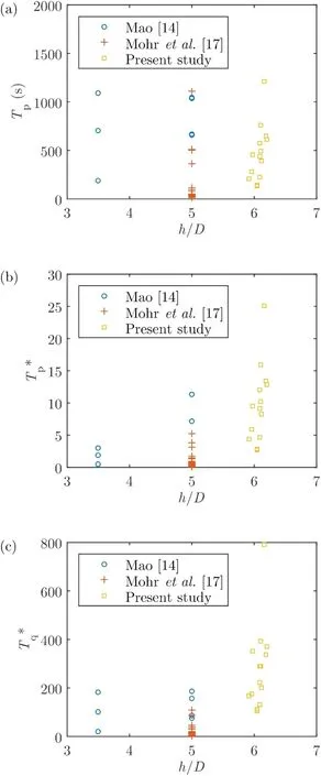
Fig. 12. Correlation between the water depth or blockage ratio, h / D , and:(a) the dimensional scour time scale, T p , which was estimated using Eq. (3) [18 , 19] ; (b) the non-dimensional scour time scale, T p ∗, which was calculated using Eq. (6) [9] ; and, (c) a new non-dimensional form of the scour time scale, T q ∗, which was calculated using ( 9 ).

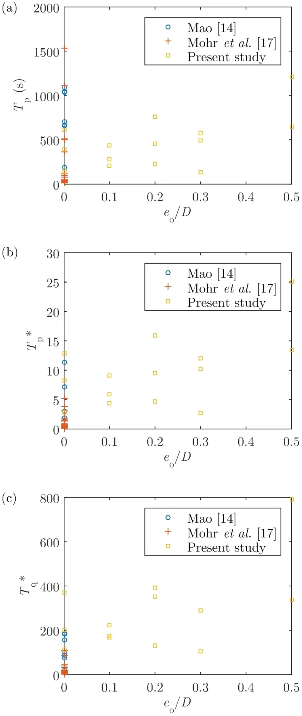
Fig. 13. Correlation between the pipe elevation ratio, e o / D , and: (a) the dimensional scour time scale, T p , which was estimated using Eq. (3) [18 , 19] ;(b) the non-dimensional scour time scale, T p ∗, which was calculated using Eq. (6) [9] ; and, (c) a new non-dimensional form of the scour time scale,T q ∗, which was calculated using Eq. (9) .

Fig. 14. Comparing the non-dimensional scour time scale, T p ∗, based on experimental data, with the values predicted using: (a) the equation proposed in Zhang et al. [18] ; (b) Eq. (17) ; and, (c) Eq. (18) . Subsequently, a new non-dimensional form of the scour time scale, T q ∗, was applied, and the experimental values were compared with the values predicted using: (d) Eq. (19) ; (e) Eq. (20) ; and finally, (f) Eq. (21) , which was seen to attain the highest correlation.

Fig. 14 presents the correlation between the empirical equations described in Section 2.2 with all clear-water and live-bed experimental data which were obtained in the present study and from published literature [14 , 17] . Fig. 14 a shows that fitting the equation proposed in [18] with the original coefficients to the experimental data had resulted in a low squared correlation coefficient. Fig. 14 b shows the correlation between the equation proposed in [18] , but with the constants updated via the optimization process described in Section 2.2 ,with the experimental data:

whereR2= 0.18, suggesting that there is a lack of consideration of other essential parameters and/or the formulation of the equation can be improved. Fig. 14 c shows the correlation of Eq. (8) with the experimental data, where the original equation was proposed in [22] , but for predicting the scour time scale beneath pipelines with partial embedment. Hence,the constants have been updated to better reflect the influence of the pipe elevation ratio,eo/D:

where the correspondingR2was approximately 0.49.

Subsequently, Eq. (9) was proposed in this work and was used to non-dimensionalise the time scale, instead of using Eq. (6) which was proposed in [9] . Fig. 14 d shows the correlation between the following equation and the experimental data:

whereby the formulation of this equation was similar to that of Eq. (17) , but the way in which the scour time scale was non-dimensionalized was modified (i.e. usinginstead of), and by using the same optimization process described in Section 2.2 , new values for the constants were computed to attain the best possible correlation (i.e.R2= 0.33). Although the correspondingR2of 0.33 for Eq. (19) is still relatively low, it is significantly improved as compared to that of Eq. (17) (i.e.R2= 0.18). In Fig. 14 e, the following equation was also seen to produce a much improved correlation with the experimental data:

whereR2= 0.64. The formulation of Eq. (20) was adopted from Eq. (18) , for which it was similar to the case for Eq. (19) wherewas used instead of, and a higher correlation was achieved. This trend has been the motivation behind developing a new equation for predicting the nondimensional scour time scale, which was based oninstead of. The following equation was formulated, as described in Section 2.2 :

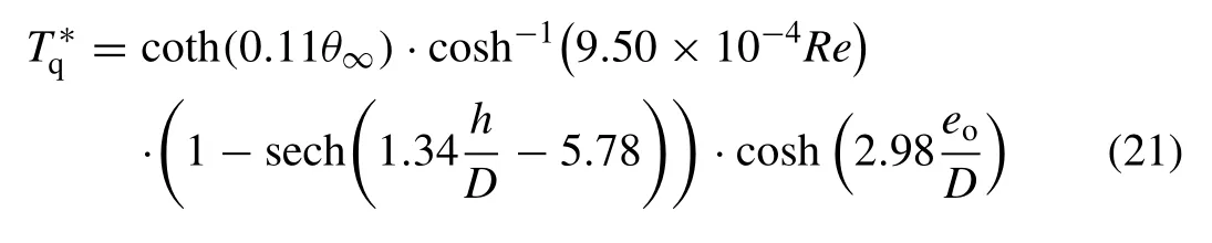
Fig. 15. Seabed gaps, G s / D , predicted using Eq. (13) , which are superimposed on the range of measured seabed gaps for the Tasmanian Gas Pipeline(TGP) [24] (shaded in grey); the upper limit of the current speed (i.e.0.79 m/s) is the maximum speed for five year return period storms [34] .

where a good correlation with the experimental data was achieved (i.e.R2= 0.74), as seen in Fig. 14 f. It appeared that Eq. (21) can be used to predict the scour time scale for pipelines with an elevation from the seabed under steady currents. Although the constant associated with the Reynolds number is small, this is the first time where the influence of the Reynolds number on the time scale had been quantified.

3.3. Field predictions

Fig. 15 compares the range of measured seabed gaps,which were obtained for the Tasmanian Gas Pipeline (TGP)[24] , with the seabed gaps that were predicted by adding the pipe elevation and the predicted equilibrium scour depths (i.e.Gs=eo+Seq); the term definitions are illustrated in Fig. 1 .The predictions for the equilibrium scour depth were made by inputting a range of current velocities and the pipe elevation ratio into Eq. (13) , based on: an external pipe diameter,D, of 0.5 m; mean sediment grain size,d50, of 0.257 mm, where thed50of the sediment that were sampled in the surveyed zone ranged from approximately 0.166 mm to 0.411 mm; mean water depth of 23 m; and, boundary layer thickness of 1 m. It is worth mentioning that by ranging thed50from 0.166 mm to 0.411 mm, the predicted maximumSeq/Dforeo/D= 0 only differed by 0.3%. Unfortunately, as the boundary layer profile was not available, a boundary layer thickness of 1 m was selected as it was assumed to be a typical boundary layer thickness over the seabed [33] . The vertical limits of the shaded area in Fig. 15 represents the range of maximum seabed gaps for every detected free span along the surveyed section of the TGP. The horizontal limit of the shaded area corresponded to a current speed of 0.79 m/s, which is the maximum speed for five year return period storms in the Bass Strait [34] . A large portion of the predicted values appear to be within the range of measured seabed gaps, and the predicted seabed gaps seem to remain constant after 0.8 m/s, at which the equilibrium scour depth would no longer increase with higher current speeds.

Fig. 16. Dimensional scour time scales, T p , predicted using Eq. (21) and Eq. (9) for the TGP.

Fig. 16 presents the predicted scour time scales for the TGP for different current speeds and pipe elevations, which were calculated using Eq. (21) , and converted into a dimensional form via Eq. (9) . The assumptions made were similar to the aforementioned assumptions which were used to predict the seabed gaps. It is worth mentioning that it was not practical to physically measure the scour time scale beneath the TGP, and hence the predicted time scales could not be compared with field measurements. Nevertheless, the time required for substantial scour to develop beneath the TGP was predicted to be longer for largereo/Dratios, and shorter for higher current speeds, generally. The predicted scour time scale for the TGP was seen to be on the order of hours, instead of minutes which was observed in the sediment flume experiments. Qualitatively, this difference in the scour time scales between the model-scale and full-scale conditions is consistent with the finding in [5] , wherein a numerical model was employed to model scour at different scales.

4.Discussion

The experimental results suggest that the pipe elevation ratio,eo/D, does have a significant influence on the development of scour beneath subsea pipelines under steady currents (i.e.both the equilibrium scour depth and the scour time scale).Wheneo/Dwas increased, smaller equilibrium scour depths were observed ( Table 4 ), whilst the maximum scour depth occurred ateo/D= 0. This can be correlated to weaker flow amplification underneath the pipe aseo/Dincreases, and thus leading to a decrease in the maximum seabed shear stress beneath the pipe [4 , 24] . In terms of the scour time scale,a general increase was observed with the increase ineo/D.This could also be attributed to the decrease in the amplified seabed shear stresses underneath the pipe aseo/Dincreases,where a reduction in the seabed shear stress would result in a lower sediment transport rate, as they are directly proportional to each other [35, 36] , and the sediment transport rate had been linked to the scour time scale [18] .

With reference to Fig. 13 , it is interesting to note that both the dimensional and non-dimensional scour time scale were observed to be slightly higher wheneo/D= 0, as compared to the time scale for the case ofeo/D= 0.1. This could have stemmed from the different mechanics of scour, or the way in which scour was initiated, for these two conditions.Wheneo/D≤0, there would initially be a flow-induced pressure difference between the upstream and downstream sides of the pipe, which promotes fluid flow through the voids in between the sediment particles beneath the pipe (i.e. seepage flow). Eventually, a mixture of water and sediment will be discharged at the immediate downstream side of the pipe (i.e.piping) [37] . This is followed by a “jet period”(i.e. tunnel erosion) where sediment is syphoned violently underneath the pipe [14] . As more sediment is eroded, the scour hole will deepen; however, wheneo/D＞ 0, the existing gap in between the pipe and the seabed would induce flow amplification, and subsequently, scour would occur underneath the pipe, provided that the local amplified seabed shear stress had exceeded the critical shear stress for the sediment. Therefore,the difference in the aforementioned mechanisms at play is thought to result in the difference in the scour time scale,where a longer period would be required for the scouring rate to reach a significant level foreo/D= 0, as compared to the case ofeo/D= 0.1.

There seem to be a significant scatter in the results in Fig. 13 . This could be attributed to other parameters that pose a strong influence on the scour time scale. For example, the upstream dimensionless seabed shear stress, θ∞. A nonlinear decrease in the scour time scale was observed as θ∞increased, as shown in Fig. 10 , whilst the scour time scale would generally increase with an increase ineo/D. On the subject of θ∞, the overall trends shown in Fig. 10 agreed with previous findings [9 , 18] . This strong relationship between the scour time scale and θ∞had led to the development of previous empirical equations [9 , 18 , 22] , in which the θ∞term was always present. This downward trend can be related to the aforementioned relationship between the seabed shear stress and the sediment transport rate, whereby an increase in θ∞would lead to an increase in the seabed shear stress underneath the pipe, and hence a higher sediment transport rate.

In this work, the adoption of a hyperbolic cotangent function in Eq. (21) for describing the relationship between the newly-derived dimensionless scour time scale,, and θ∞was seen to contribute towards achieving a good correlation with the experimental data overall (i.e.R2= 0.74). As this work had contributed significant clear-water experimental data, whilst previous work [9 , 18 , 22] largely focused on the live-bed condition, Eq. (21) , which was fitted to both conditions, can therefore be used for predicting the scour time scale both under clear-water and live-bed conditions. Eq. (21) is introduced in an attempt of simplification, whereby a single equation is proposed for both clear-water and live-bed conditions. In contrast, Dogan and Arisoy [15] found different dependencies of the non-dimensional scour time scale, and proposed two separate equations for the clear-water and livebed conditions. Therefore, a possible improvement in the correlation between the equation proposed in this work and the experimental data may be attainable by having two separate equations.

In addition to the strong relationship between the scour time scale and θ∞, the θ∞term was also included in Eq. (21) as it has been successfully adopted for scaling laboratory experiments that involve sediment transport for many years [38] . On the topic of scale effects, another important parameter to consider is the Reynolds number,Re[39] . However, a relatively weak relationship betweenandRewas observed, based on the results shown in Fig. 11 as well as the small constant in Eq. (21) . This occurrence was expected,asRewas previously found to pose a small influence on the maximum seabed shear stress beneath the pipe and the equilibrium scour depth [4] .

The water depth ratio,h/D, was seen to have an effect on the non-dimensional scour time scale. Although the relationship between the dimensional scour time scale,Tp, andh/Dwas relatively unclear ( Fig. 12 a), the non-dimensional scour time scale was seen to increase with the increase inh/D( Fig. 12 b and c). A previous numerical study [32] , in which the influence ofh/Dwas investigated independent of other variables, reported that the time required for the equilibrium scour depth to be achieved was approximately 2.9 times higher whenh/D= 10, as compared toh/D= 2.5. However,it seemed that this could not be validated with experimental data due to the physical limitations associated with laboratory setups, where having highh/Dratios would not be possible.In addition, higherh/Dratios were neither investigated experimentally nor numerically, and the upper limit at whichh/Dno longer poses an influence on the dimensionless scour time scale is still an unknown, whilst the equilibrium scour depth was seen to initially decrease and tend towards a constant value despite a further increase inh/D( Fig. 6 ). Nevertheless, Eq. (21) was formulated in such a way that the nondimensional scour time scale will not tend towards infinity whenh/Dapproaches infinity. It is hypothesised that a comprehensive multi-phase numerical model would be required to systematically study the effect of having large water depths on the scour time scale beneath full-scale subsea pipelines(e.g.h/D＞ 100).

A new manner of non-dimensionalising the scour time scale, via Eq. (9) , was seen to improve the correlation of existing empirical equations to the compilation of experimental data ( Fig. 14 ). In comparison to Eq. (6) [9] , Eq. (9) proposed the removal of the indices, or powers (e.g.D2), which would alter the units of certain parameters (e.g. from m to m2).However, a flux parameter (i.e.Uo) was introduced in Eq. (9) ,which was not present in Eq. (6) . This flux parameter,Uo, was mainly introduced to normalize the time scale without relying on indices. The presence of multiple powers in Eq. (6) was hypothesized to result in “overfitting”in a sense.

With reference to Fig. 16 , the dimensional scour time scale for the Tasmanian Gas Pipeline (TGP) was predicted to increase witheo/D, suggesting that the time required for substantial scour to develop would be longer for higher pipe elevations, which can be related to the reduction in the aforementioned seabed shear stress amplification factor. The time scale was seen to generally decrease with an increase in the current speed, and approach a certain value; however, there was an initial increase in the time scale at low current speeds,which was followed by a rapid change, at which a maximum value was reached. This could be related to the formulation of Eq. (21) , wherein an increase in the current speed would influence both θ∞andRe. The time scale would tend to decrease with an increase in θ∞, whilst the time scale would tend to increase with an increase inRe, but the constants in Eq. (21) suggest that the influence of θ∞is more significant than that ofRe; however, the increase in the scour time scale with the flow velocity was also observed in the sediment flume experimental results ( Table 4 ), where an occasional decrease in the scour time scale was observed; this inconsistency was also observed in [9] . Nevertheless, the increase in the scour time scale was observed to occur at very low current speeds in Fig. 16 (i.e. less than 0.1 m/s), and thus,we conclude that the dimensional scour time scale would generally decrease with the current speed.

Although the scour time scale could not be compared with field measurements, the influence of the pipe elevation on the scour time scale had not been investigated in previous work.In addition, full-scale predictions have also been made for the seabed gaps ( Fig. 15 ), for which the predictions made using Eq. (13) appeared to be mostly within the range of measured values in [24] . It is worth mentioning that the highest incidence in terms of the measured seabed gaps was found to beGs/D= 0.5, at more than 35%, which was followed byGs/D= 0.6, and subsequently, small ratios (i.e.Gs/D＜ 0.5)[24] . However, the scour depths beneath the TGP may not necessarily be in an equilibrium state. Therefore, it can only be deduced that there seemed to be a correlation between the predictions made using Eq. (13) and the measured values,while the scour depth may deepen if it is not in equilibrium.In addition, along the surveyed section of the TGP, the seabed has been observed to be mostly comprised of uniform sand,but occasionally, rocks have been observed. Thus, the seabed gaps could be present due to scouring beneath the pipe and/or feature mobility where the seabed is uneven.

In summary, the compilation of experimental data in this work suggests that the non-dimensional scour time scale is significantly influenced by the upstream dimensionless bed shear stress, θ∞, and the pipe elevation ratio,eo/D, whilst the effect of the Reynolds number is small, and the effect of the water depth or blockage ratio,h/D, can be further investigated with sophisticated numerical models without physical restrictions in terms of the size of the computational domain. As previous experimental investigations on the scour time scale largely focused on live-bed conditions and bottom-seated or partially embedded pipelines, this work presents Eq. (21) , in which the scour time scale was non-dimensionalized using a new formulation as shown in Eq. (9) , that is found to result in a high correlation to the experimental data. Eq. (21) is applicable for pipelines with an elevation with respect to the far-field seabed under steady currents, as well as both clearwater and live-bed conditions.

5.Summary and conclusions

This work focused on predicting the scour time scale beneath subsea pipelines with an elevation with respect to the far-field seabed under steady currents. A range of pipe elevation ratios, 0 ≤eo/D≤ 0.5, were considered for the sediment flume experiments, and additional experimental data from published literature were compiled as well. Equations have been formulated to non-dimensionalize the time scale,and to predict the time scale as a function of the upstream seabed shear stress, θ∞, Reynolds number,Re, water depth ratio,h/D, andeo/D. The following major conclusions have been drawn based on the results presented in this work:

·A general increase in the scour time scale was observed aseo/Dincreased.

·The effect ofReon the time scale was small.

·The non-dimensional time scale was seen to increase with an increase inh/D; however, the dimensional time scale does not appear to be affected byh/D.

·A new form of the non-dimensional scour time scale,which is calculated using Eq. (9) , was found to aid the empirical equations in attaining a better correlation to the experimental data.

·A new empirical equation, Eq. (21) , is proposed for predicting the non-dimensional scour time scale beneath pipelines with aneo/Dunder steady currents, which has a good correlation with experimental data, and is applicable for both clear-water and live-bed conditions.

·As the scour time scale for the TGP was not known, the measured scour depths beneath the full-scale pipeline may not be at equilibrium. Nevertheless, the comparison between the seabed gaps predicted using Eq. (13) and the field measurements did not indicate that the full-scale predictions are erroneous.

Acknowledgments

The authors thank Katie Stagl, Jasmin McInerney, Bill Sluis, and Daret Kehlet, for their kind assistance with the sediment flume experimental setup.