
Explicit Symplectic Geometric Algorithms for Quaternion Kinematical Differential Equation
2018-05-02 07:11HongYanZhangZiHaoWangLuShaZhouQianNanXueLongMaandYiFanNiu
Hong-Yan Zhang,Zi-Hao Wang,Lu-Sha Zhou,Qian-Nan Xue,Long Ma,and Yi-Fan Niu
I.INTRODUCTION
QUATERNIONS,invented by the Irish mathematician W.R.Hamilton in 1843,have been extensively utilized in physics[1],[2]aerospace and aeronautical technologies[3]-[12],robotics and automation[13]-[17],human motion capture[18],computer graphics and games[19]-[21],molecular dynamics[22],and flight simulation[23]-[26].Quaternions have no inherent geometrical singularity as Euler angles when parameterizing the 3-dimensional special orthogonal group manifold SO(3,R)with local coordinates and they are useful for real-time computation since only simple multiplications and additions are needed instead of trigonometric relations.Almost all of the researches available about the applications of quaternions focus on these two merits and the fundamental quaternion kinematical differential equation(QKDE)[1],[3],[8].In[1],Robinson presented the following QKDE
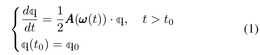
wheret0is the initial time,ω=[ω1(t),ω2(t),ω3(t)]Tis the angular velocity vector,=[e0,e1,e2,e3]Tis the matrix representation of the quaternionwith scalar parte0as well as vector part[e1,e2,e3]T,and
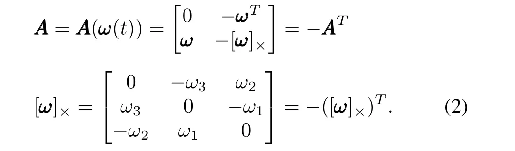
Formally,(1)is a linear ordinary differential equation(ODE)and its numerical solution should be easily determined in practical engineering applications.However,as Wie and Barbar[3]pointed out,the coefficientsω1,ω2,ωT3,or equivalently the angular rate vectorω=[ω1,ω2,ω3],are time-varying and the matrixAAAhas the repeated eigenvalues
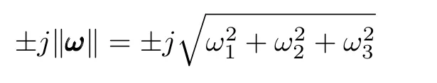
where‖·‖denotes theℓ2-norm.This implies that the linear time-varying system,i.e.,the QKDE described by(1),is critically(neutrally)stable and the numerical integration is sensitive to the computational errors.Therefore,it is necessary to find a robust and long time precise integration method for solving(1).Many researchers have studied this problem with the traditional finite difference method since 1970s.Hrastar[27],Cunninghamet al.[28]and Wie and Barbar[3]used the Taylor series method.Miller[29]tried the rotation vector concept.Mayo[30]adopted the Runge-Kutta[31]and the state transition matrix method.Wang and Zhang[32]compared the Runge-Kutta scheme with symplectic difference scheme,and Fundaet al.[14]used the periodic normalization to unit magnitude.However,even for the time-invariantω,the traditional numerical schemes for QKDE are sensitive to the accumulative computational errors in the sense of long time term.
In the past 30 years,the symplectic geometric algorithms(SGA)were originally proposed by Feng[33]and Ruth[34]independently and developed systematically by other researchers[35]-[39].The advantage of SGA is that it can be used to solve the Hamiltonian system efficiently with a non-dissipative numerical scheme which avoids accumulative computational errors.For the ODE of time-varying system,the Gauss-Legendre(G-L)difference scheme[40],[41],an accurate and implicit Runge-Kutta method,is an implicit symplectic geometric algorithm(ISGA)essentially.However,it needs an extra iterative process to solve the numerical solution(NS).Its computational complexity isO(n2)[42]and thus,it is not appropriate for real-time applications.
We solve(1)via explicit symplectic geometric algorithms(ESGA)which overcomes the disadvantages of traditional non-symplectic difference schemes and symplectic GL method.Firstly,we consider the autonomous QKDE(AQKDE)with constant parametersω1,ω2andω3.The A-QKDE can be modelled with autonomous Hamiltonian system and solved by the SGA.Secondly,we discuss the non-autonomous QKDE(NA-QKDE)whereω1(t),ω2(t),ω3(t)depend on time explicitly and design ef ficient difference scheme with symplectic method.
The main purpose of this paper is to propose ESGAs for solving the general NA-QKDE while preserving long time precision and the norms of quaternions automatically with linear time computation complexity.The contents of this paper are organized logically.The preliminaries of ESGA are presented in Section II.Section III deals with the ESGA for the A-QKDE.In Section IV we cope with the ESGA for NA-QKDE.The simulation results are presented in Section V.Finally,Section VI gives the summary and conclusions.
II.PRELIMINARIES
A.Hamiltonian System
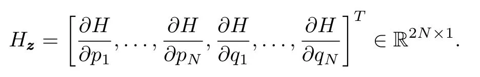
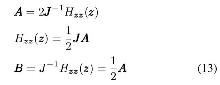
W.R.Hamilton introduced the canonical differential equations[43],[44]
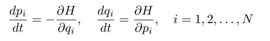
for problems of geometrical optics,wherepiare the generalized momentums,qiare the generalized displacements andH=H(p1,...,pN,q1,...,qN)is the Hamiltonian,viz.,the total energy of the system.Letthenspecified byzzzin the 2N-dimensional phase space.Since the gradient ofHis
Then,the canonical equation is equivalent to
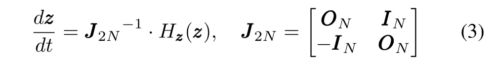
whereIINis theN×Nidentical matrix,OOONis theN×Nzero matrix andJJ2Nis the 2Nth order standard symplectic matrix[33],[37].For simplicity,the subscripts inIIN, II2NandJJJ2Nmay be omitted.Any system which can be described by(3)is called a Hamiltonian system.There are some fundamental properties for the canonical equation of Hamiltonian system[43],[45]-[47]:
1)it is invariant under the symplectic transform(phase lf ow);
2)the evolution of the system is the evolution of symplectic transform;
3)the symplectic symmetry and the total energy of the system can be preserved simultaneously and automatically.
B.Transition Matrix
The SGA was motivated by the three fundamental properties 1)-3).Ruth[34]and Feng[33]emphasized two key points in their pioneering works:
a)SGA is a kind of difference scheme which preserves the symplectic structure of Hamiltonian system;
b)the single-step transition matrix is a symplectic transform(matrix)which preserves the symplectic structure of the difference equation(discrete version)of the continuous form of(3).
Letτbe the time step andzzz[k]=zzz(t0+kτ)be the sample value at the discrete timetk=t0+kτ.With the initial condition

the symplectic difference scheme(SDS)for(3)is given by
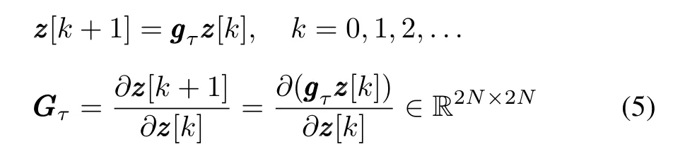
wheregggτ:R2N×1→R2N×1is the transition operator,also named the transition mapping,andGGGτis the transition matrix(Jacobi matrix)ofggτatzzz[k]such thatGτis symplectic,viz.,

Equivalently,we haveGGGτ∈Sp(2N,R)⊂GL(2N,R)⊂R2N×2N,in which Sp(2N,R)is the symplectic transform group and GL(2N,R)is the general linear transform group[48]-[50].When designing SGA,the key problem is to determine thegggτor its Jacobi matrixGGGτsince both of them can be used to construct the SDS of interest.In this paper,we will find the symplectic matrixGGGτand we always havegτ=GGτsince(1)is a linear ODE.
For the general non-linear and non-separable Hamiltonian system,the centered Euler implicit scheme(CEIS)is a widely used SGA with second order precision.It is described by[37]

in which the midpointis de fined by
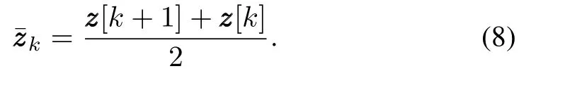
The CEIS can be used to find the transition matrixGGGτ.Let
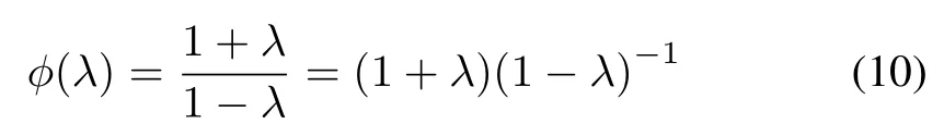
be the Cayley transform.Then,for smallτsuch thatis non-singular,we have[37]
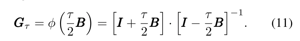
Note that although(11)is an approximate result in the sense of approximate conservation[33]for the general non-linear Hamiltonian system(linear Hamiltonian system requires that the Hessel matrixHzzzz(·)is symmetric),it could be a precise solution for some special cases.
III.SYMPLECTIC ALGORITHM FOR A-QKDE
A.A-QKDE and Autonomous Hamiltonian System
When the matrixAAin(1)is time-invariant,or equivalently the parametersω1,ω2andω3are constants,we can model(1)with the autonomous Hamiltonian system.PuttingN=2,pppwe can obtain
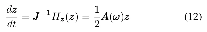
by(1)and(2).We remark here that the notationzzzis usually used in the literatures about SGA while notationis used in references about quaternions.The equivalence shows thatandzzcan be used alternatively if necessary.From(12)we can find thatTherefore
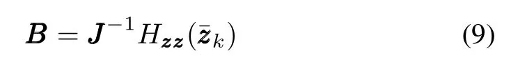
according to(9).Note thatJJJAA/=AA JJ,so the Hessel matrixHzzzzzz(zzz)is not symmetric,which means that the Hamiltonian system here is nonlinear by definition[37].Obviously,the AQKDE is an autonomous Hamiltonian system and the SGA can be adopted.
B.Symplectic Transition Matrix
We now prove some interesting lemmas and theorems for constructing the SDS for A-QKDE.
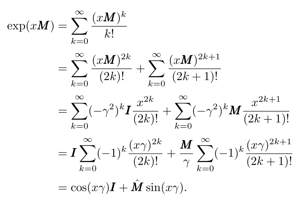
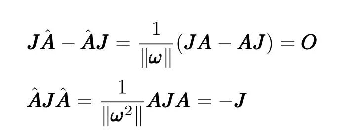
Lemma 1(Generalized Euler’s formula):Suppose matrixMMM∈Rn×nis skew-symmetric,i.e.,MMMT=-MMM,andˆ there exists a positive constantγsuch thatMMM2=-γ2II.LetMMM=γ-1MMM,then=- III.For anyx∈R,we have

Proof:
Lemma 2(Cayley-Euler formula):Suppose matrixMMM∈Rn×nis skew-symmetric,i.e.,MMM2T=-MMM,and there exists apositiveconstantγsuch thatMMM=-γ2II.Let=γ-1MMM,then=- III.Letφ(λ)be the Cayley transformation,then for anyx∈R the Cayley-Euler formula

holds,in whichθ=θ(x,γ)=2·arctan(xγ)andα=x2γ2.Furthermore,φ(xMMM)is an orthogonal matrix.
Proof:It is trivial thatanyx∈R,we find thatIn consequenceHence the Cayley transformationφ(xMMM)can be simplified as following
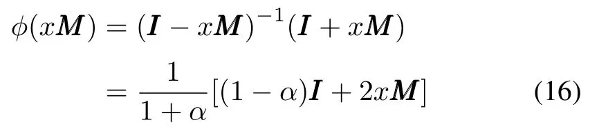
whereα=x2γ2.Let tan(θ/2)=xγ,then by the trigonometric identity,MMM=γˆMMMand Lemma 1,we immediately have
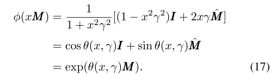
Moreover,
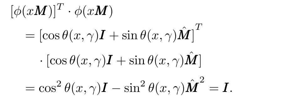
Similarly,we can obtainφ(xMMM)·[φ(xMMM)]T=III.Henceφ(xMMM)is orthogonal by definition. ¥
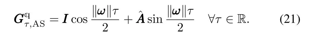
Theorem 1:For any time stepτand time-invariant vectorω,the transition matrixfor the A-QKDE is
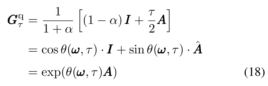
in whichα=τ2‖ ω‖2/16,θ=2arctan(τ‖ ω‖/4),
Proof:With the help of(11)and(13),the transition matrix will be.Letx=τ/4,MMM=AAA,γ=‖ ω‖,thenα=x2γ2=‖ ω‖2τ2/16.Thus the theorem follows from Lemma 2 directly.
Theorem 2:For anyω∈R3×1andτ∈R,the transition matrixis an orthogonal transformation and an invertible symplectic transformation with second order precision,i.e.,
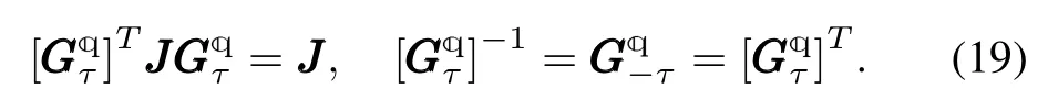
Proof:For a constant vectorω,we can find the functionθ=2arctan(τ‖ ω‖/4)is an odd function of time stepτ.By utilizingwe immediately obtain
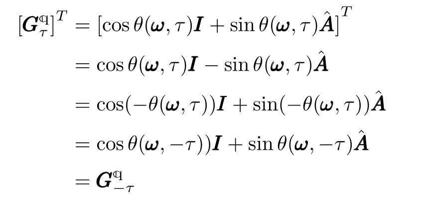
which implies that the transition matrix is invertible.Moreover,is orthogonal by Lemma 2.In consequence,Furthermore,simple algebraic operation implies that
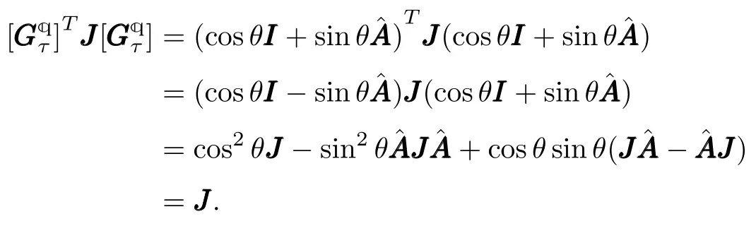
Henceis a symplectic matrix.Since theis constructed from CEIS directly,it must be a second order precision scheme. ¥
C.Comparison With Analytic Solution
Fortunately,the analytic solution(AS)for A-QKDE can be found without difficulty.In fact for anyt∈[t0,tf]wheret0andtfdenote the initial and final time respectively,we have
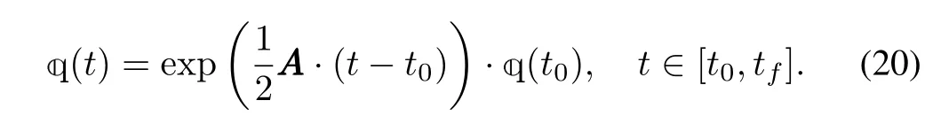
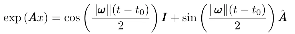
by Lemma 1.Thus fort-t0=τ,the AS to the transition matrix for the A-QKDE is
At the same time,for sufficiently smallτin(18)we have
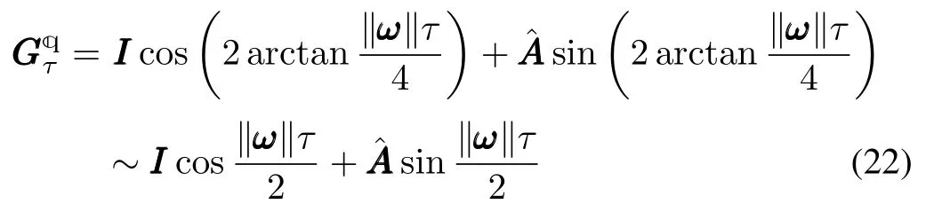
for sufficiently smallx=‖ ωτ‖since
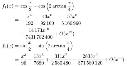
Letr=maxx∈R+{|f1(x)|,|f2(x)|},then we haver<1.25×10⁻⁴forx≤0.2 andr<1.57×10⁻⁸forx≤0.01.Therefore,thecan be approximated by with an acceptable precision when time stepτ≤1/(5‖ ω‖).
D.Explicit Symplectic Geometric Algorithm for A-QKDE
The ESGA for A-QKDE based on CEIS,ESGA-I for brevity,is given in Algorithm 1 by the explicit expression ofobtained.
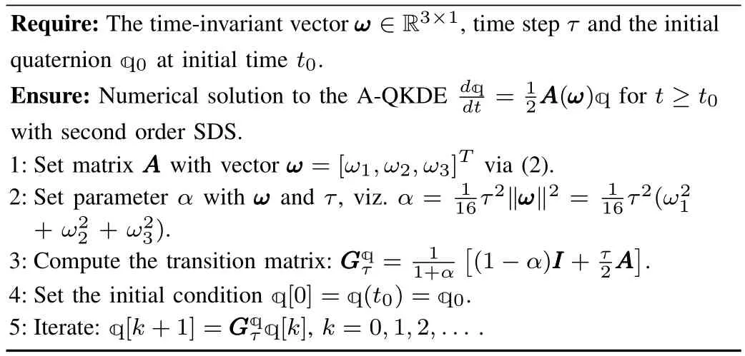
Algorithm 1 Explicit Symplectic Geometric Algorithm for A-QKDE(ESGA-I)
Suppose that the time consumed for the multiplication and addition of real numbers areδ1andδ2,respectively,the function invoking time is ignored and there areniterations in Step 5.Table I shows that the total time consumed(without optimization)is 20(2δ1+δ2)+(16δ1+12δ2)n=O(n).Therefore,the time complexity is linear.Moreover,we have tostoreω1,ω2,ω3, AAA,τ,α, ,kand[k].Note that all of the[k]share a common storage and only 43 real numbers should be stored in this algorithm.Obviously,the space complexity is constant,i.e.,O(1).

TABLE ITIME AND SPACE CONSUMPTIONS OF ESGA-I
IV.SYMPLECTIC GEOMETRIC METHOD FOR NA-QKDE
A.Time-dependent Parameters and NA-QKDE
For the time-varying vectorω=ω(t),(1)implieszzz˙=whereH=H(p1,p2,q1,q2,t)=H(e0,e1,e2,e3,t).Hence the NA-QKDE is a non-autonomous Hamiltonian system essentially and the corresponding SGA can be obtained via the concept of extended phase space[37].Letp3=h,q3=t,wherehis the negative of the total energy.Letzzz=[p1,p2,h,q1,q2,t]T=[pppT,h, qqT,t]T∈R(2N+2)×1,K(zz˜z)=h+H(p1,p2,q1,q2,t)=h+H(ppp, qqq,t)=h+H(,t),then we have the time-centered Euler implicit scheme(T-CEIS)with fourth order[37],
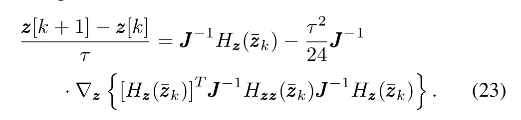
Equation(23)shows that for the time-varying problems,H∗()is replaced byH∗()where∗may beppp,qqqort.In order to gTuarantee the duality of the phase space,we takezzz=[ppT, qqqT].The symplectic scheme for the NA-QKDE as(23)can be simplified as
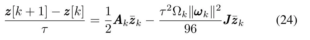

By taking the similar procedure as we do in finding the transition matrix for SDS of the A-QKDE,we can obtain
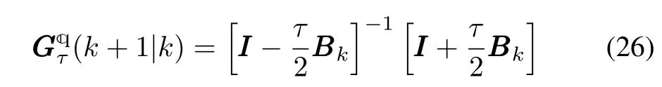
whereBBBkis a skew-symmetric matrix such that
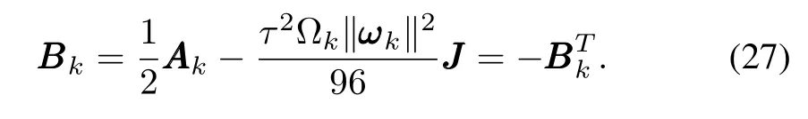
According to Lemma 2,there exists a series ofγksuch that
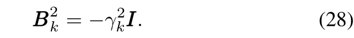
Theorem 3:For the NA-QKDEthen fork=0,1,2,...,the transition matrixwill be
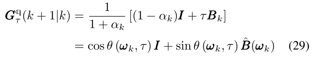
such that

whereθ=2arctan
We remark that this SDS is a fourth order scheme according to[37].In addition,sinceω(t)is time-dependent andω(t[k]-τ/2)/=ω(t[k]+τ/2)for positiveτin general,we can deduce thatalthoughis also a symplectic and orthogonal transformation.
B.Explicit Symplectic Geometric Scheme for NA-QKDE
The ESGA for NA-QKDE based on T-CEIS,ESGA-II for brevity,is presented in Algorithm 2.With the similar complexity calculations for Algorithm 1,we can find that the time complexity and space complexity of Algorithm 2 are alsoO(n)andO(1),respectively.
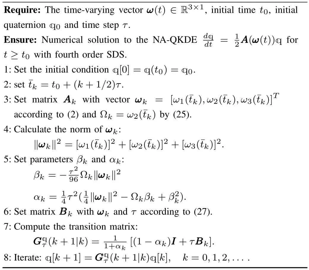
Algorithm 2 Explicit Symplectic Geometric Algorithm for NAQKDE(ESGA-II)
We remark here thatωk=ω(¯tk)=ω(t[k]+τ/2)relates the fractional interval sampling,which will increase the complexity of the hardware implementation.However,if the sampling ratefs=1/τis large enough,theω(t)will vary slowly in each short time interval[t[k],t[k+1]]and the linear interpolation can be considered here.This is to say that fort∈[t[k],t[k+1]]
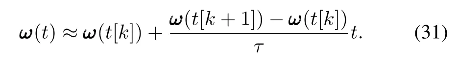
Hence
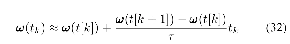
with acceptable precision.In this way the fractional interval sampling can be avoided and the complexity of the hardware implementation can be reduced.
V.NUMERICAL SIMULATION
A.Key Issues for Verification and Validation
Although the algorithms are designed according to the proved lemmas and theorems,it is still necessary to verify them with concrete examples by numerical simulation.Unfortunately,each quaternion has four components,thus it is not convenient for visualization.However,it is still possible to check the algorithms proposed with the following facts:
1)the norm can be used as a necessary condition for validating the correctness of the algorithms proposed sincethe transition matricesare orthogonal and the norm of the quaternions should be preserved as‖(t)‖=1;
2)the relation of stability,accumulative errors and time step of ESGA can be compared with other numerical methods;
3)the asymptotic behavior can be identified clearly whenω(t)approaches to a constant vector(thus the NA-QKDE may degenerate to A-QKDE asymptotically);
4)for some special cases,we can compare the AS and NS conveniently;
5)the time complexity of ESGA and ISGA can be compared for the same NA-QKDE and con figuration of parameters.
For A-QKDE,theωis time-invariant andω=‖ ω‖is a constant.Since the eigen-values of matrixAAA(ω)are±jω,then the general solution to A-QKDE must be

in which the amplitudesciand phasesφican be determined by the initial condition.
For NA-QKDE,if we choose the functionsω2(t)andω3(t)such that for sufficient larget,ω2(t)→0 andω3(t)→0,then(1)shows that there existst∗∈R such that
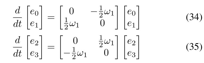
fort>t∗since=[e0,e1,e2,e3]T.Hence(t)+(t)=(0)+(0)and(t)+(t)=(0)+(0)asymptotically.Ifω1(t)→aasymptotically(whereais a constant),then we have
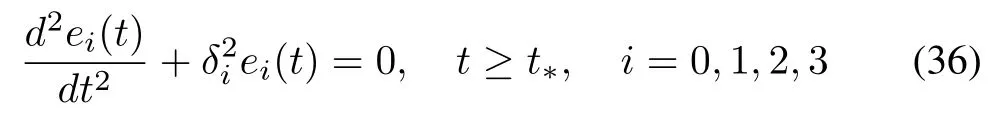
whereδi=a/2.In other words,eachei(t)can be described by(33)asymptotically.
Without loss of generality,we can set the initial condition as(0)=[1,0,0,0]Tfor the verification,thus we just need to considere0(t)ande1(t).Letand tanthen Lemma 2 implies that

whereθ=2arctan(ω1()τ/4).Obviously,is a symplectic matrix by(6).
B.Numerical Examples
We now demonstrate the intuitive ideas and show the performance of ESGA with concrete examples.All of the numerical experiments in this subsection are implemented in MATLAB and run on a desktop PC equipped with IntelCoreTMi7-3770 CPU@3.4GHz and 4GB RAM.
1)Numerical Solution vs.Analytical Solution:Fig.1 illustrates the performance of ESGA-II with an AS.We set the parameters asω0=2π,β=π/80,initial state[0]=[cos(β/2),0,sin(β/2),0]and such that the AS is
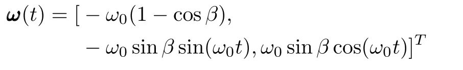
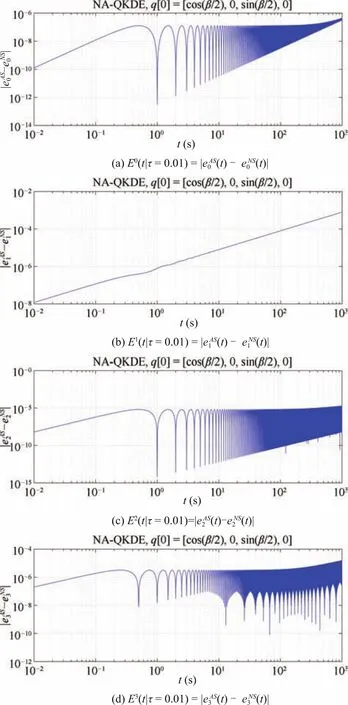
Fig.1.Absolute errors of NS by Algorithm 2(SGA-NA-QKDE)with ω0=2π,β = π/80,τ =0.01s,t0=0,tf=1000s.
The absolute value of error between the NS and AS for theith component and fixed time step is de fined by

Ei(t|τ)is computed with ESGA-II for eachei(t),see Fig.1.We find that all these errors of NS are stable and small when the time stepτ=0.01 second(a low data sampling rate)and time duration is 1000 seconds.This implies that the accuracy and stability of SGA remain well for NA-QKDE.
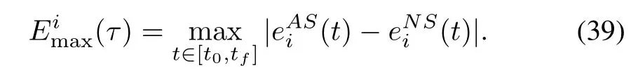
2)Asymptotic Performance—Connection of A-QKDE and NA-QKDE:Fig.2 demonstrates the asymptotic performance of ESGA for QKDE.We find that for differentω(t),we have‖(t)=1‖for anytand there are no accumulated errors.On the other hand,the solutions to QKDE will have different properties for differentω(t):
a)In Fig.2(a),eachei(t)is a cosine function sinceωiis a constant according to(33).
b)In Fig.2(b),e0(t)ande1(t)vary like cosine curves asymptotically becauseω1(t)→0 asymptotically.Moreover,it is trivial thate2(t)=e3(t)≡0 sinceω2(t)=ω3(t)≡0 ande2(0)=e3(0)=0 by(35).
c)In Fig.2(c),ω1(t)→2,ω2(t)→0,ω3(t)→0 whent→∞.It is easy to find that eachei(t)varies periodically whent>10 by(36).We remark that att=0,ω2(0)/=0,ω3(t)/=0,which leads to positive feedbacks fore2(t)ande3(t)and the increasing of their amplitudes.
d)In Fig.2(d),ω(t)has no asymptotic behavior but it is periodic.Although eachek(t)varies independently,we still have(t)≡1.
3)Stability,Accumulative Errors and Time Step:Fig.3 shows the precision and stability with the time step.We find that the four-stage explicit Runge-Kutta(RK4)method works well only when the time step is small and the time duration is relatively short(about 15s),otherwise the norm cannot be kept well.Furthermore,the Euler-Backward(EUB)method always leads to serious accumulative errors.Fortunately,both ESGA and ISGA work well and there is no computational damp since the norm‖‖remains constant.
4)Computational Complexity—ESGA vs.ISGA(G-L Method):Fig.4 represents the time complexity of ESGA for NA-QKDE in comparison with that of ISGA,i.e.,G-L method.We solved the(1)with the same parametersω(t)and[0]as that in Fig.1.For each fixed time stepτand componentei(t),the maximum error is de fined by
The maximum errors and computing time of the two methods are calculated with different time stepτ.Although the precision of ESGA is worse than that of ISGA for the same time step,the time complexity of ESGA is far lower than that of G-L method.For example,the time consumed in G-L method is about 10 times of our ESGA as shown in the figure forτ=0.01.Actually,the computing time of ESGA is almost less than 1 second for most cases in our experimental setup,however it is about 7s for the G-L method.This implies that the ESGA is much better than ISGA if the time consumption is a key issue for hardware or software implementation.The linear time complexityO(n)of our algorithms is essential for the real-time applications such as navigation and control system.
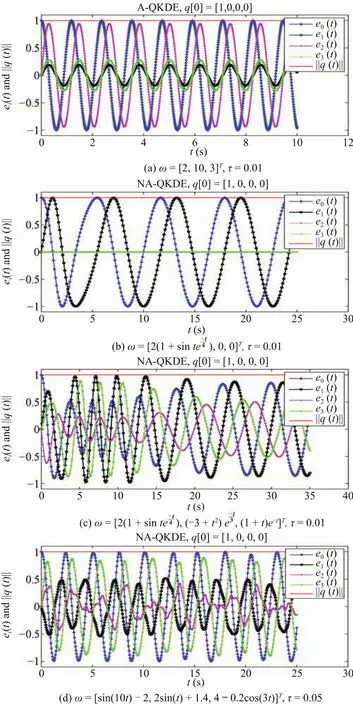
Fig.2. NS to QKDE for different ω(t)and[0]=[1,0,0,0]T.
VI.CONCLUSIONS
In this paper we proposed a key idea of solving the QKDE with symplectic method:each QKDE can be described by an autonomous or non-autonomous Hamiltonian system and the CEIS or T-CEIS can be used to design ESGA for QKDE.The generalized Euler’s formula and Cayley-Euler formula for the symplectic transition matrix play a key role in designing ESGAs with first and second order precision.The correctness and efficiencies of the ESGAs presented are verified and demonstrated by asymptotic analysis and comparison with AS and NS.
Fig.3.Performances of SGA,RK4 and EUB for NA-QKDE with periodic ω(t)=[sin(10t)-2,2sin(t)+1.4,4-0.2cos(3t)]T.
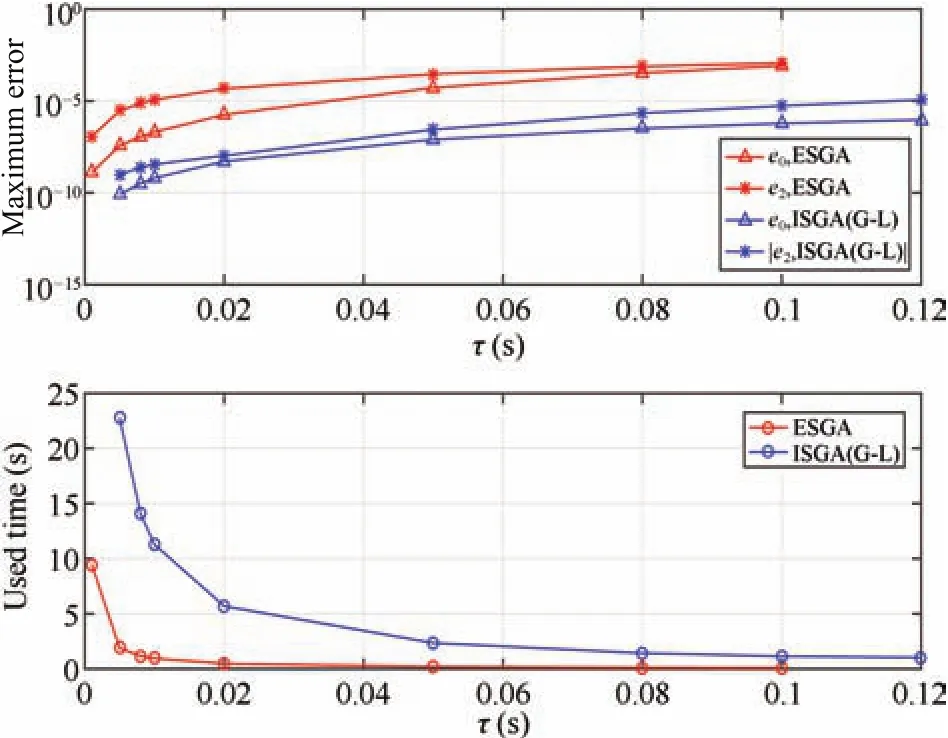
Fig.4.Maximum errors E0max(τ)and E2max(τ),and computing time of ESGA-II and ISGA(G-L method)with ω0=2π,β = π/80,t0=0,tf=500s.
Compared with the traditional difference scheme such as RK4 and EUB,our ESGA-I for A-QKDE and EGSA-II for NA-QKDE are symplectic and can avoid the accumulative errors in the sense of long time term.On the other hand,our explicit symplectic method is better than the implicit symplectic method because of its linear time complexity and potential applications for real-time systems.
As part of future work,we will investigate the high-order precision ESGA for QKDE,the robustness of ESGA-II perturbed by noise,the applications of ESGA to more general linear time-varying system and its combination with precise-integration method.Additionally,we will also design second order precision symplectic-precise integrator to solve the linear quadratic regulator problem and the matrix Ricatti equation since they play an important role in automation.
ACKNOWLEDGMENT
The first author would like to thank Prof.Daniel Dalehaye of Ecole Nationale de l’Aviation Civile because part of this work was carried out while this author was visiting ENAC.We are indebted to Prof.Yi-Fa Tang whose lectures on symplectic geometric algorithms for Hamiltonian system at Chinese Academy of Sciences attracted the first author and stimulated this work in some sense.The authors’thanks go to Ms.Fei Liu,Mr.Jing-Tang Hao and Ms.Ya-Juan Zhang for correcting some errors in an earlier version of this paper.
[1]A.C.Robinson,“On the use of quaternions in simulation of rigid-body motion,”Wright Air Development Center,Tech.Rep.,Dec.1958.
[2]Y.J.Lu and G.X.Ren,“A symplectic algorithm for dynamics of rigid body,”Appl.Math.Mech.,vol.27,no.1,pp.51-57,Jan.2006.
[3]B.Wie and P.M.Barba,“Quaternion feedback for spacecraft large angle maneuvers,”J.Guid.Contr.Dynam.,vol.8,no.3,pp.360-365,May 1985.
[4]B.Wie,H.Weiss,and A.Arapostathis,“Quarternion feedback regulator for spacecraft eigenaxis rotations,”J.Guid.Contr.Dynam.,vol.12,no.3,pp.375-380,May 1989.
[5]B.Wie and J.B.Lu,“Feedback control logic for spacecraft eigenaxis rotations under slew rate and control constraints,”J.Guid.Contr.Dynam.,vol.18,no.6,pp.1372-1379,Nov.1995.
[6]B.Wie,D.Bailey,and C.Heiberg,“Rapid multitarget acquisition and pointing control of agile spacecraft,”J.Guid.Contr.Dynam.,vol.25,no.1,pp.96-104,Jan.2002.
[7]J.Kuipers,Quaternions and Rotation Sequences:A Primer with Applications to Orbits,Aerospace and Virtual Reality.Princeton:Princeton University Press,2002.
[8]B.Friedland,“Analysis strapdown navigation using quaternions,”IEEE Transactions on Aerospace and Electronic Systems,vol.AES-14,no.5,pp.764-768,Sep.1978.
[9]A.Kim and M.F.Golnaraghi,“A quaternion-based orientation estimation algorithm using an inertial measurement unit,”inPosition Location and Navigation Symp.,2004,Monterey,CA,USA,USA,2004,pp.268-272.
[10]R.Rogers,Applied Mathematics in Integrated Navigation Systems(third edition).Virginia,USA:AIAA,2007.
[11]Y.M.Zhong,S.S.Gao,and W.Li,“A quaternion-based method for SINS/SAR integrated navigation system,”IEEE Trans.Aerosp.Electron.Syst.,vol.48,no.1,pp.514-524,Jan.2012.
[12]M.Zamani,J.Trumpf,and R.Mahony,“Minimum-energy filtering for attitude estimation,”IEEE Trans.Automat.Contr.,vol.58,no.11,pp.2917-2921,Nov.2013.
[13]J.S.Yuan,“Closed-loop manipulator control using quaternion feedback,”IEEE J.Robot.Automat.,vol.4,no.4,pp.434-440,Aug.1988.
[14]J.Funda,R.H.Taylor,and R.P.Paul,“On homogeneous transforms,quaternions,and computational efficiency,”IEEE Trans.Robot.Automat.,vol.6,no.3,pp.382-388,Jun.1990.
[15]J.C.K.Chou,“Quaternion kinematic and dynamic differential equations,”IEEE Trans.Robot.Automat.,vol.8,no.1,pp.53-64,Feb.1992.
[16]O.-E.Fjellstad and T.I.Fossen,“Position and attitude tracking of AUV’s:a quaternion feedback approach,”IEEE J.Oceanic Eng.,vol.19,no.4,pp.512-518,Oct.1994.
[17]J.T.Cheng,J.Kim,Z.Y.Jiang,and W.F.Che,“Dual quaternionbased graphical SLAM,”Robot.Autonom.Syst.,vol.77,pp.15-24,Mar.2016.
[18]D.S.Alexiadis and P.Daras,“Quaternionic signal processing techniques for automatic evaluation of dance performances from MoCap data,”IEEE Trans.Multim.,vol.16,no.5,pp.1391-1406,Aug.2014.
[19]F.Dunn and I.Parberry,3D Math Primer for Graphics and Game Development.Texas:Word Ware Publishing Inc.,2002.
[20]D.H.Eberly,3D Game Engine Design:A Practical Approach to Realtime Computer Graphics(Second Edition).Boca Raton:CRC Press,2006.
[21]J.Vince,Quaternions for Computer Graphics.London:Springer,2011.
[22]T.Miller III,M.Eleftheriou,P.Pattnaik,A.Ndirango,D.Newns,and G.J.Martyna,“Symplectic quaternion scheme for biophysical molecular dynamics,”J.Chem.Phys.,vol.116,no.20,pp.8649-8659,May 2002.
[23]J.M.Cooke,M.J.Zyda,D.R.Pratt,and R.B.McGhee,“NPSNET:flight simulation dynamic modeling using quaternions,”Presence:Teleoper.Virt.Environ.,vol.1,no.4,pp.404-420,1992.
[24]D.Allerton,Principles of Flight Simulation.Wiltshire,UK:John Wiley&Sons,2009.
[25]D.J.Diston,Computational Modelling and Simulation of Aircraft and the Environment,Volume 1:Platform Kinematics and Synthetic Environment.Wiltshire,UK:John Wiley&Sons,2009.
[26]J.S.Berndt,T.Peden,and D.Megginson,“JSBSim,open source fl ight dynamics software library,”[Online].Available:http://jsbsim.sourceforge.net/,Jan.9,2017.
[27]J.Hrastar,“Attitude control of a spacecraft with a strapdown inertial reference system and onboard computer,”NASA,Tech.Rep.,Sep.1970.
[28]D.C.Cunningham,T.P.Gismondi,and G.W.Wilson,“Control system design of the annular suspension and pointing system,”J.Guid.Contr.Dynam.,vol.3,pp.11-21,May 1980.
[29]R.B.Miller, “A new strapdown attitude algorithm,”J.Guid.Contr.Dynam.,vol.6,no.4,pp.287-291,Jul.1983.
[30]R.A.Mayo, “Relative quaternion state transition relation,”J.Guid.Contr.Dynam.,vol.2,pp.44-48,May 1979.
[31]J.C.Butcher,“Coefficients for the study of Runge-Kutta integration processes,”J.of the Australian Math.Soc.,vol.3,no.2,pp.185-201,1963.
[32]S.J.Wang and H.Zhang,“Algebraic dynamics algorithm:Numerical comparison with Runge-Kutta algorithm and symplectic geometric algorithm,”Sci.China Ser.G:Phys.Mech.Astronom.,vol.50,no.1,pp.53-69,Feb.2007.
[33]K.Feng, “On difference schemes and symplectic geometry,”inProc.1984 Beijing Symp.Differential Geometry and Differential Equations,Beijing,China,1984,pp.42-58.
[34]R.D.Ruth, “A canonical integration technique,”IEEE Trans.Nuclear Sci.,vol.30,no.4,pp.2669-2671,Mar.1983.
[35]K.Feng and M.Z.Qin,“Hamiltonian algorithms for Hamiltonian systems and a comparative numerical study,”Comput.Phys.Commun.,vol.65,no.1-3,pp.173-187,Apr.1991.
[36]L.H.Kong,R.X.Liu,and X.H.Zheng,“A survey on symplectic and multi-symplectic algorithms,”Appl.Math.Comput.,vol.186,no.1,pp.670-684,Mar.2007.
[37]K.Feng and M.Z.Qin,Symplectic Geometric Algorithms for Hamiltonian systems.Berlin Heidelberg:Springer,2010.
[38]J.M.Sanz-Serna and M.P.Calvo,Numerical Hamiltonian problems.London:Chapman and Hall/CRC,1994.
[39]E.Hairer,C.Lubich,and G.Wanner,Geometric Numerical Integration:Structure-Preserving Algorithms for Ordinary Differential Equations.Berlin Heidelberg:Springer,2006.
[40]J.C.Butcher, “Implicit Runge-Kutta processes,”Math.Comput.,vol.18,no.85,pp.50-64,Jan.1964.
[41]A.Iserles,A First Course in the Numerical Analysis of Differential Equations.Cambridge:Cambridge University Press,1996.
[42]J.M.Varah,“On the efficient implementation of implicit Runge-Kutta methods,”Math.Comput.,vol.33,no.146,pp.557-561,1979.
[43]V.I.Arnold,Mathematical Methods of Classical Mechanics.New York:Springer,1989.
[44]V.I.Arnold,V.V.Kozlov,and A.I.Neishtadt,Mathematical Aspects of Classical and Celestial Mechanics.Berlin Heidelberg:Springer,2006.
[45]L.H.Kong,J.L.Hong,L.Wang,and F.F.Fu,“Symplectic integrator for nonlinear high order Schr¨odinger equation with a trapped term,”J.Comput.Appl.Math.,vol.231,no.2,pp.664-679,Sep.2009.
[46]J.Franco and I.G´omez,“Construction of explicit symmetric and symplectic methods of Runge-Kutta-Nystr¨om type for solving perturbed oscillators,”Appl.Math.Comput.,vol.219,no.9,pp.4637-4649,Jan.2013.
[47]D.M.Hernandez,“Fast and reliable symplectic integration for planetary systemN-body problems,”Mon.Not.R.Astronom.Soc.,vol.458,no.4,pp.4285-4296,Jun.2016.
[48]V.Guillemin and S.Sternberg,Symplectic Techniques in Physics.Cambridge:Cambridge University Press,1990.
[49]S.Sternberg and Y.Li,Lectures on Symplectic Geometry.Tsinghua University Press,2012.
[50]A.C.da Silva,Lectures on Symplectic Geometry.Berlin Heidelberg:Springer,2008.
 IEEE/CAA Journal of Automatica Sinica2018年2期
- IEEE/CAA Journal of Automatica Sinica的其它文章
- Decomposition Methods for Manufacturing System Scheduling:A Survey
- Nonlinear Bayesian Estimation:From Kalman Filtering to a Broader Horizon
- Vehicle Dynamic State Estimation:State of the Art Schemes and Perspectives
- Coordinated Control Architecture for Motion Management in ADAS Systems
- An Online Fault Detection Model and Strategies Based on SVM-Grid in Clouds
- An Adaptive RBF Neural Network Control Method for a Class of Nonlinear Systems