
Takagi-Sugeno fuzzy model identification for turbofan aero-engines with guaranteed stability
2018-06-28 11:04RuichoLIYingqingGUOSingKiongNGUANGYifengCHEN
CHINESE JOURNAL OF AERONAUTICS 2018年6期
Ruicho LI,Yingqing GUO,*,Sing Kiong NGUANG,Yifeng CHEN
aSchool of Power and Energy,Northwestern Polytechnical University,Xi’an 710129,China
bDepartment of Electrical and Computer Engineering,The University of Auckland,Auckland 1142,New Zealand
1.Introduction
Turbofan aero-engine,designed to work safely and efficiently under a wide range of operating conditions,plays a pivotal role in the flight capabilities of modern aircrafts.To achieve a consistent transient response under a variety of working con-ditions,the gain scheduling technology is utilized extensively in engine control systems.The main idea of gain scheduling is to decompose the complex nonlinear aero-engine system into a set of linear systems by selecting break points.Then controllers are designed for each break point to cover all the operating conditions.As a consequence,a large number of break points have to be selected such that the system behavior between adjacent breakpoints is applicable for linear interpolations.Moreover,due to the lack of a systematic method,designs and validations of the controllers are still exhausting efforts.To facilitate the controller design,the Takagi-Sugeno(TS)fuzzy control is found to be a promising solution which motivates us to establish a TS fuzzy model for the aero-engine.
The TS fuzzy model proposed by Takagi and Sugeno1is described by the following IF-THEN rules which represent the local input-output relationship of a nonlinear system:
IF antecedent proposition THEN consequent proposition.Then the overall system is achieved by fuzzy blending of these local models.Generally,a TS fuzzy model is established by linearizing the given nonlinear model around its operating points.However,as in many engineering applications,an explicit mathematical model of the aero-engine is very hard to obtain.Thus,the data-driven identification method is preferred in this paper.
When performing identification,antecedents and consequents of the rules are usually identified separately.Among them,efforts are made majorly on the latter by various methods,like fuzzy clustering2,3or evolving methods.4–6This is because with fixed antecedent parameters,identifying parameters of the consequent models is formulated as a linear leastsquare problem,which can be solved analytically and optimally.7However,in existing studies8–11and references therein,only Nonlinear AutoRegressive eXogenous(NARX)types are considered as the form of the consequents.To the best of our knowledge,the state-space representation which is favored in most control relevant studies has not been formulated so far.
Besides,due to reasons like non-persistent exciting signals,measurement noises or even inappropriate partitions of the antecedent space,the identified model may be unstable.However,only a little attention has been paid on the stability of the identified fuzzy systems.Among them,Abonyi et al.12transforms the prior-knowledge of the process stability into linear inequality constraints when identifying a TS fuzzy system of the NARX type.As for the identification of linear models,methods like augmenting the data13or the cost function14have been developed to obtain a stable representation at a cost of distorting the data or the cost function.By contrast,Lacy and Bernstein15guarantees the stability by introducing additional constraint.As a result,a specific weighting matrix should be taken therein.However,this is not a common case since the weighting matrix usually has a physical meaning and therefore cannot be designated casually.Inspired by Lacy and Bernstein’s method,stability constraints of innovative forms are proposed in this paper for the TS fuzzy system,which includes the local linear system as a special case.
To sum up,the contribution of this paper is threefold.First,given fixed antecedent parameters,the problem of identifying a TS fuzzy system of state-space representation is formulated and has not been established before.Then based on this representation,a new theorem is proposed to ensure the global asymptotic stability of the identified TS fuzzy system and all its local models.Finally,the proposed method is utilized to identify a TS fuzzy system for the turbofan aero-engines,which facilitates the application of the fuzzy control.
This paper is organized as follows:the preliminary is presented in Section 2,and identifying the TS fuzzy system with guaranteed stability is formulated in Section 3.Then numerical example of a turbofan aero-engine is given in Section 4.Finally,conclusion is presented in Section 5.
2.Preliminary
The ith local discrete linear model of the TS fuzzy model can be described as follows:

where i=1,2,...,Nris the rule index,z= [z1,z2,...,zNz]∈ RNzis the premise variables vector and Mi1,Mi2,...,MiNzare corresponding fuzzy sets.x(k)∈ RNxis the state vector.u(k)∈ RNuis the input vector.y(k)∈ RNyis the measured output vector.(δx,δy,δu)denotes the deviation from the ith steady-state point value
By using weighted average defuzzifier,these local models are integrated into a global nonlinear model as follows.The instant index k of z(k)is omitted in the following when there is no ambiguity.

where


where Mip(zp)(p=1,2,...,Nz)is the degree of membership function of zpin the fuzzy set Mip.Following the practice in most control relevant studies,throughout this paper triangular membership functions are utilized and are arranged in a gridtype manner.For a better understanding,the product of two triangular membership functions and the grid-type partition of rules are shown in Fig.1 respectively.
Problem formulation:in this paper,we focus on identifying the consequent parameters(the system matrices of each rule)with structures of the antecedents and the consequents(namely the number of rules Nr,the partition of the antecedent space and the dimensions Nz,Nx,Nyand Nu)being determined in advance based on a prior-knowledge.With this assumption,problem of identifying the TS fuzzy system is summarized as:
Given: firing strength μi(z)(i=1,2,...,Nr)and measured sequences δujl(k), δxjl(k)and δyjl(k)in which the subscript‘jl” denotes the lth (l=1,2,...,Nl)measurement sampled under the jth (j=1,2,...,Ndata) flight condition.
Determine:stable local system matrices Gi,Hi,Ciand Di(i=1,2,...,Nr)which guarantee the stability of the overall TS fuzzy system.
3.Identification of the consequent parameters with guaranteed stability
Given structures of the antecedents and the consequents,problem of estimating the consequent parameters is formulated and presented in this section.Besides,to ensure the stabilities of the overall identified fuzzy system and all its local models which are known in advance,additional constraints are introduced further in form of Linear Matrix Inequalities(LMIs).Then combining the aforementioned work,solution to the problem in preliminary is presented.
3.1.Identification as a least-square problem
The identification method used in this paper is an extension of the subspace system identification method.16In the conventional subspace identification method,the system matrices G(zj),H(zj),C(zj)and D(zj)of different operating points(premise variables)zj(j=1,2,...,Ndata)are estimated separately(or called locally)by minimizing a cost function based on the one-step-ahead prediction error as

where Wjlis the weighting matrix with diagonal structures,Yjland Vjlare augmented matrices defined as


Fig.1 Product of two membership functions and grid-type partition.
It can be seen each group of data are only used for a local interpretation and thus the fuzzy relationship Eq.(3)between system matrices of adjacent operating points(premise variables)is not established.
To establish the fuzzy relationship,all the local models are identified simultaneously in one optimization as follows.By substituting Eq.(3)into Eq.(5)and adding them up,the fuzzy identification problem is formulated as minimizing an object defined below.

where

It can be seen that J(Λ)is a quadratic object of which the minimum can besolved analytically by the following proposition:
Proposition 1.The least-square solution of minΛJ(Λ)is

Proof.By the property of Frobenius norm,J(Λ)can be expanded as

the derivative of which is
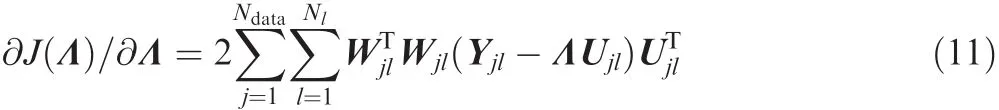
Then based on vec(ABC)= (CT⊗ A)vec(B),by taking∂J(Λ)/∂Λ =0 and performing vectorization on both sides,we obtain
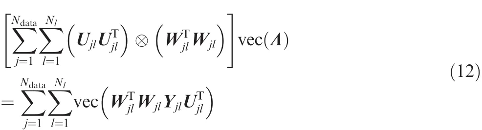
of which the least-square solution is Eq.(9).The proposition is proved.□
3.2.Stability of identified fuzzy model
Although parameters of the consequent models are estimated analytically as mentioned above,the obtained model can be unstable undesirably.As mentioned in introduction,the requirement of stability is transformed into constraints to stabilize the models.To achieve this,the fuzzy system Eq.(1)is rewritten first as follows.
Assume the antecedent space is partitioned into a set of individual subspaces.Denote the partition as Rswhere s=1,2,...,Nsis the subspace index.In the sth subspace Rs,the fuzzy system Eq.(1)can be expressed as

withi∈I(s)μi(z)=1.I(s)is a set which contains all the indexes of system matrices firing in the sth subspace Rs.Based on the form of Eq.(13),a lemma is introduced below which ensures the global asymptotic stability of the TS fuzzy system.
Lemma 117.The TS fuzzy system Eq.(13)is globally exponentially stable if there exist a set of symmetric Pssuch that the following constraints are satisfied,

where set A(s)contains the index s and all the indexes of subspaces being adjacent to sth the subspace Rs.
Remark 1.Lemma 1 is adopted from the Ref.17.The distinction lies in the range of q which is restricted to the set A(s)defined here.This is because in a practical application it is assumed the premise variables always change continuously due to their physical property,which means they only transit between the adjacent subspaces and cannot jump into a nonadjacent subspace.
Remark 2.The overall TS fuzzy system being stable does not necessarily require all its local models to be stable.But for a practical plant,its local model is usually known to be stable as a prior-knowledge.Thus,we favor the lemma above to develop the follow-up work as it containsi<0 as a special case,which is the stability condition of the ith local model(Gi,Hi,Ci,Di),i=1,2,...,Nr.
It is noted that Eq.(14)are not convex constraints because neither Gi(i∈ I(s))nor Pq(q ∈ A(s))is known in advance when performing identification.To transfer constraints Eq.(14)into numerically tractable forms,the following theorem is proposed.
Theorem 1.The TS fuzzy system Eq.(13)is globally exponentially stable if there exist a set of symmetric matrices Psand a matrix F such that the following LMIs are satisfied.

Proof.By applying Schur complement to Eq.(14)and performing congruence transformation with a block diagonal matrix diag(I,F),it can be known that the TS fuzzy system is globally exponentially stable if there exist a set of positive definite matrices Ps> 0(s=1,2,...,Ns)such that

holds.Then based onwe have,the theorem is proved.□
Remark 3.The proof is similar to the Ref.18.However,the theorem therein is applied in control synthesis to express the controller design as LMIs.To the best knowledge of the authors,this is the first time the approach is utilized in an identification problem,where both the Lyapunov matrix Pqand system matrix Giare undetermined.
In Theorem 1,an auxiliary matrix F is introduced to decouple the Lyapunov matrix Pqwith the system matrix Gi.Hence by imposing constraints Eq.(15)on the object Eq.(7),the global stability of the identified model is guaranteed.As a byproduct mentioned in Remark 2,the stability of each consequent local model is also ensured.Summarizing the work above,the solution to the problem proposed in Section 2 is given below.
Problem solution:solution to the problem proposed above,namely identifying a TS fuzzy system with guaranteed stability,is formulated as a quadratic programing problem with positive-semidefinite constraints as

which can be solved efficiently by existing optimization solvers.
4.Numerical examples
In this section,a TS fuzzy model with guaranteed stability is identified for turbofan aero-engines working under the maximum power status(non-afterburning).Different power status can also be modeled by the same method through incorporating inputs/outputs/states as premise variables.However,in that case,the antecedent space is high-dimensional and hence cannot be displayed graphically.For a better understanding,this section focuses on a particular power status over the flight envelope.Readers should keep in mind that the proposed method is generic which can be applied to a more complex case.This section is arranged as follows:the working principle of turbofan aero-engines is described brie fly first.Then structures of the fuzzy model are determined based on a priorknowledge and data are collected for identification.Finally,the fuzzy system is identified and effectiveness of the stability constraints is presented.
4.1.Mixed- flow two-spool turbofan aero-engines
Cross-section of the mixed- flow two-spool turbofan aeroengine is given in Fig.2.For a two-spool bypass turbofan engine,two compressors and two turbines are linked by concentric shafts,which rotate independently,namely the Low-Pressure Compressor(LPC)is driven by the Low-Pressure Turbine(LPT)and the High-Pressure Compressor(HPC)is powered by the High-Pressure Turbine(HPT).
Before we go further,notations of the antecedent and consequent parameters and their physical meanings are summarized in Table 1 for a quick reference.
4.2.Determination of antecedent structure
To prevent the engine from exceeding its structural and aerodynamic operating limits,the allowable flight conditions(namely the Mach number Ma and the altitude Alt)are restricted to the so-called flight envelope,which is a closed region as shown in Fig.3(assuming a nominal sea-level temperature).
Since the aero-engine is designed to operate reliably over an extended range of flight conditions,it is natural to regard theflight envelope as the antecedent space and select Ma and Alt as the premise variables vector z,namely

Table 1 Notation of antecedent and consequent parameters.

Fig.2 Cross-section of a mixed- flow two-spool turbofan aero-engine.

Fig.3 Flight envelope and its partition.

Based on this choice,by taking the number of rules as Nr=62and applying an even grid-type partition,the flight envelope is partitioned into Ns=52subspaces as shown in Fig.3.For an intuitive understanding,premise variables( flight conditions) satisfying μi(z)=1(i=1,2,...,Nr) are also denoted in blue circles in Fig.3.They are exactly the maximum points of Fig.1(b).It should be highlighted that a different number of rules or other partitions of the antecedents are still applicable and may even bring a higher fitting accuracy.But they are designated directly here because obtaining an optimal antecedent structure is not the focus of this paper.
4.3.Determination of consequent structure
In this section,structure of the consequent part,including the dimensions and physical meanings of the states,inputs and outputs,is determined based on an expert knowledge.
Generally,mechanical system dynamics due to rotating inertias constitutes the most important contribution to the engine transient behavior.Therefore,the low-pressure shaft speed NLand the high-pressure shaft speed NHare usually selected as the states as

Furthermore,to obtain a maximum power,the engine usually switches between different control modes,which means the inputs and the controlled outputs vary when operating in a different region within the flight envelope.
Following the switching logic of the turbofan areo-engine AЛ-31Φ,19a combined control mode is applied in this paper,which works depending on the sub-regions depicted in Fig.3.This combined control mode is taken as:

Considering the control modes listed above,the input vector u and the controlled output vector y are taken as

which consist of all the possible inputs and outputs.Thus,the turbofan aero-engine operating under different control modes is expressed in a uniform form for the convenience in identification.
Besides,steady-state values of the tripleunder each flight condition zj(j=1,2,...,Ndata)are also designated.However,they vary with the flight condition and thus are too trivial to list here.Readers who are interested could consult the Ref.19for more details.
4.4.Data collection
The data used in this paper are generated from the aerothermodynamics component-level model of a mixed- flow two spool turbofan aero-engine.20Readers who are interested in the modeling principle could obtain more details from Ref.21.
In this section,two samples are collected under each flight condition zj(j=1,2,...,Ndata).The engine model is first driven to the jth steady-stateand then two excitation sequences δujl(k)(l=1,2)are added separately to the inputsto generate the derivation sequences δxjl(k)and δyjl(k).These two excitation sequences are taken respectively as

in which ‘chirp” is a swept-frequency cosine signal with amplitude being 1%,ω(k)is a zero-mean white Gaussian sequence of which the Signal-to-Noise Ratio(SNR)satisfies

where σnoisedenotes standard deviation of the white Gaussian noise,σsignaldenotes standard deviation of the excitation signal.
For an aero-engine,frequencies of the dominant dynamics are generally not higher than 2 Hz.22Hence frequency of the chirp function is set to increase from 0 to 2 Hz linearly to extract the dominant spectral characteristics.Also based on this prior-knowledge,the sampling period Tsis taken as 0.025 s.Consequently,the sampling frequency fs=40 Hz is more than twenty times higher than the dominant frequency and thus is adequate for control purpose.
Take the first flight condition z1= [Ma,Alt]= [0,0 km]as an example,the two samples (l=1,2)including the inputs δum,1l(m=1,2,...,Nu),the states δxn,1l(n=1,2,...,Nx)and the outputs δyr,1l(r=1,2,...,Ny)obtained under this condition are drawn in Fig.4,in which their amplitudes have already been normalized by their steady-state value.
Finally, simulation data of 287 flight conditions(Ndata=287)are collected in which each data contain two samples(Nl=2).The data are sampled every 0.1 for Ma and every 1 km for Alt as the red dots shown in Fig.3.

Fig.4 Example of simulation data.
4.5.Determination of weighting matrix
The Normalized Mean Square Error(NMSE)is a frequently used index for measuring the distinction between the fitting and the measured sequences.Take the rth output yr(k)(r=1,2,...,Ny)as an example,given reference sequence yr(k)and its fitting sequence^yr(k),the NMSE is defined as

where

The value of NMSE varies between 0(perfect fit)and∞(bad fit).If NMSE is equal to 1,then^yr(k)is no better than a straight line at matching yr(k).In this way,the relationship between the goodness of fit and the NMSE is established.
Furthermore,if the weighting matrix Wjlin Eq.(7)is taken as
where

then the object J(Λ)gains a physical meaning as the total NMSE of states and outputs over all the measurements.
4.6.Results
After determining all the related parameters and collecting data,we are ready to identify a TS fuzzy model with known stability for the turbofan aero-engine.By taking the matrix F in constraints Eq.(15)as the identity matrix I,problem Eq.(17)is solved using the YALMIP toolbox23to obtain system matrices of each rule (Gi,Hi,Ci,Di)(i=1,2,...,Nr).However,they are not listed here due to their huge amounts.Instead,NMSE over the entireflight envelope are presented in Fig.5 as a result to show the effectiveness of the proposed method.
In Fig.5,it can be seen that by selecting states based on a prior-knowledge,the states achieve high fitting accuracies with NMSE being less than 3.4×10⁻³over the entireflight envelope.In contrast,the outputs fit in an acceptable level which is generally not higher than 0.2 but still deteriorate badly under some flight conditions(as can be seen from the NMSE of y2in Fig.5(b),which may arise from an inappropriate partition of the flight envelope).
Besides,it is noted that only partial NMSE of Regions I&II are depicted in Fig.5.This is because in these regions,the outputs are not activated for feedback or the sample is generated purely from an inactivated input channel as mentioned in Section 4.3.Therefore,to improve the fitting accuracy,contributions of these measurements are eliminated by taking their weighting as 0 and thus the corresponding NMSE are meaningless to be presented.
4.7.Comparisons on stability
To demonstrate the effect of the stability constraints,value of the object J(Λ)without/with constraints are calculated simultaneously,which are 41.7666 and 41.7667 respectively.It can be seen that there is only a slight degradation in J(Λ)when constraints are introduced.

Fig.5 NMSE over entireflight envelope.
Besides,poles of the local models with/without constraints are also drawn in Fig.6.It can be observed from Fig.6(a)that when no constraint is imposed,the stability is violated slightly as one of the poles locates out of the unit disk region.This unstable system matrix is given below of which the flight condition is z= [1.2,20 km].Its poles are also marked in red in both figures for comparison.


Fig.6 Poles of system matrices Gi(i=1,2,...,Nr).
Since the aero-engine is known to be stable over the flight envelope,there is no doubt that the fuzzy system containing this unstable local model cannot represent the dynamic of aero-engine correctly.To solve this,stability constraints Eq.(15)are introduced to suppress the unstable poles as shown in Fig.6(b).The corresponding system matrix is also given below,which is now stabilized at the cost of a slight increment on the value of object J(Λ)as mentioned above.

Furthermore,a grid of constant damping factor ξ and a natural frequency line ωn=0.1π/Tsare also depicted in Fig.6.Take the sampling period Ts=0.025 s as mentioned above,it is interesting to see that natural frequencies of all the poles are lower than ωn=4π =2 Hz.This fact confirms the frequencies of the input excitation sequences are high enough to exact the dominant dynamics.
5.Conclusions
In this paper,the problem of identifying the turbofan aero-engine as a TS fuzzy model is formulated as a quadratic optimization.The stability of the identified TS fuzzy is also considered and guaranteed by incorporating positivesemidefinite constraints.Effectiveness of the proposed method is validated by numerical examples,in which the average goodness of fit reaches a high level while all the local models are stabilized with only a slight loss in the fitting accuracy.However,it is noted that the fitting accuracy of certain flight condition is still poor which can be improved by a further optimization on the antecedents.
1.Takagi T,Sugeno M.Fuzzy identification of systems and its applications to modeling and control.IEEE Trans Syst,Man,Cybernet 1985;SMC-15(1):116–32.
2.Rezaee B,Zarandi MHF.Data-driven fuzzy modeling for Takagi-Sugeno-Kang fuzzy system.Inform Sci 2010;180(2):241–55.
3.Li CS,Zhou JZ,Fu B,Kou PG,Xiao J.T-S fuzzy model identification with a gravitational search-based hyperplane clustering algorithm.IEEE Trans Fuzzy Syst 2012;20(2):305–17.
4.Askari M,Markazi AHD.A new evolving compact optimised Takagi-Sugeno fuzzy model and its application to nonlinear system identification.Int J Syst Sci 2012;43(4):776–85.
5.Lin YY,Chang JY,Lin CT.Identification and prediction of dynamic systems using an interactively recurrent self-evolving fuzzy neural network.IEEE Trans Neural Networks Learn Syst 2013;24(2):310–21.
6.Shi HB,Li XS,Hwang KS,Pan W,Xu GJ.Decoupled visual servoing with fuzzy Q-learning.IEEE Trans Indus Inform 2016;14(1):241–52.
7.Chiu SL.Fuzzy model identification based on cluster estimation.J Intell Fuzzy Syst 1994;2(3):267–78.
8.Abonyi J.Fuzzy model identification.New York:Springer Science&Business Media;2003.p.87–164.
9.Ahn KK,Anh HPH.Inverse double NARX fuzzy modeling for system identification.IEEE/ASME Trans Mechatron 2010;15(1):136–48.
10.Hellendoorn H,Driankov D.Fuzzy model identification:Selected approaches.New York:Springer Science&Business Media;2012.p.53–90.
11.Billings SA.Nonlinear system identification:NARMAX methods in the time,frequency,and spatio-temporal domains.Hoboken:John Wiley&Sons;2013.p.61–104.
12.Abonyi J,Babuska R,Verbruggen HB,Szeifert F.Incorporating prior knowledge in fuzzy model identification.Int J Syst Sci 2000;31(5):657–67.
13.Chui NLC,Maciejowski JM.Realization of stable models with subspace methods.IFAC Proc Volumes 1996;29(1):4255–60.
14.Van Gestel T,Suykens JAK,Van Dooren P,De Moor B.Identification of stable models in subspace identification by using regularization.IEEE Trans Autom control 2001;46(9):1416–20.
15.Lacy SL,Bernstein DS.Subspace identification with guaranteed stability using constrained optimization.IEEE Trans Autom Control 2003;48(7):1259–63.
16.Van Overschee P,De Moor BL.Subspace identification for linear systems:Theory-implementation-applications.New York:Springer Science&Business Media;2012.p.31–59.
17.Wang L,Feng G.Piecewise H∞controller design of discrete time fuzzy systems.IEEE Trans Syst,Man,Cybernet,Part B(Cybernet)2004;34(1):682–6.
18.De Oliveira MC,Bernussou J,Geromel JC.A new discrete-time robust stability condition.Syst Control Lett 1999;37(4):261–5.
19.Zhao DZ,Wang HD.Control schedule analysis for AЛ-31Φ aero-engine.Aeroengine 1997;(1):14–9[Chinese].
20.Zhang SG,Guo YQ,Lu J.Research on aircraft engine component-level models based on GasTurb/MATLAB.J Aerospace Power 2012;27(12):2850–6[Chinese].
21.Martin S,Wallace I,Bates DG.Development and validation of an aero-engine simulation model for advanced controller design.American control conference;2008 Jun 11-13;Seattle,USA.Piscataway:IEEE Press;2008.p.2334–9.
22.Jaw LC,Mattingly JD.Aircraft engine controls:Design,system analysis,and health monitoring.Reston:AIAA;2009.p.69–71.
23.Lofberg J.YALMIP:A toolbox for modeling and optimization in MATLAB.Proceedings of the computer aided control system design conference;Piscataway:IEEE Press;2004.p.284–9.
 CHINESE JOURNAL OF AERONAUTICS2018年6期
- CHINESE JOURNAL OF AERONAUTICS的其它文章
- An efficient aerodynamic shape optimization of blended wing body UAV using multi- fidelity models
- Effect of multiple rings on side force over an ogive-cylinder body at subsonic speed
- Dynamic temperature prediction of electronic equipment under high altitude long endurance conditions
- Experimental investigation on static/dynamic characteristics of a fast-response pressure sensitive paint
- Experimental study on film cooling performance of imperfect holes
- Mechanism of stall and surge in a centrifugal compressor with a variable vaned diffuser